
| |
 在 Github 上查看源代码 在 Github 上查看源代码
|
|
|
在此 CoLab 笔记本中,您将学习如何使用 TensorFlow Lite Model Maker 来训练自定义音频分类模型。
Model Maker 库能够使用迁移学习来简化使用自定义数据集训练 TensorFlow Lite 模型的过程。使用您自己的自定义数据集重新训练 TensorFlow Lite 模型可以减少所需的训练数据量,并将缩短训练时间。
这是在 Android 上自定义并部署音频模型 Codelab 中的一部分。
您将使用一个自定义的鸟类数据集,并导出一个可在手机上使用的 TFLite 模型、一个可用于在浏览器中进行推断的 TensorFlow.JS 模型,以及一个可用于服务的 SavedModel 版本。
安装依赖项
sudo apt -y install libportaudio2pip install tflite-model-maker
导入 TensorFlow、Model Maker 和其他库
在所需的依赖项中,您将使用 TensorFlow 和 Model Maker。除了这些,其他依赖项用于音频操作、播放和可视化。
import tensorflow as tf
import tflite_model_maker as mm
from tflite_model_maker import audio_classifier
import os

import numpy as np
import matplotlib.pyplot as plt
import seaborn as sns

import itertools
import glob
import random

from IPython.display import Audio, Image
from scipy.io import wavfile

print(f"TensorFlow Version: {tf.__version__}")
print(f"Model Maker Version: {mm.__version__}")
TensorFlow Version: 2.9.1
Model Maker Version: 0.4.0
Birds 数据集
Birds 数据集是 5 种鸟类歌声的教育集合:
- White-breasted Wood-Wren(白胸林鹩)
- House Sparrow(家麻雀)
- Red Crossbill(红交嘴雀)
- Chestnut-crowned Antpitta(栗顶蚁鸫)
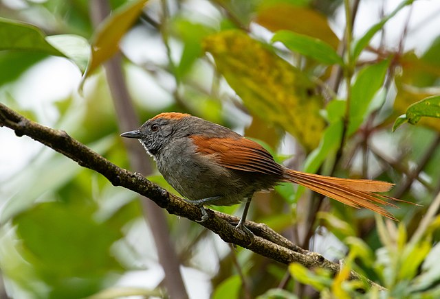
- Azara's Spinetail(阿氏针尾雀)
原始音频来自 Xeno-canto,这是一个致力于分享世界各地鸟鸣的网站。
我们从下载数据开始。
birds_dataset_folder = tf.keras.utils.get_file('birds_dataset.zip',
                                                'https://storage.googleapis.com/laurencemoroney-blog.appspot.com/birds_dataset.zip',
                                                cache_dir='./',
                                                cache_subdir='dataset',
                                                extract=True)
Downloading data from https://storage.googleapis.com/laurencemoroney-blog.appspot.com/birds_dataset.zip
343680986/343680986 [==============================] - 3s 0us/step
探索数据
音频已被拆分为训练文件夹和测试文件夹。在每个拆分的文件夹中,每种鸟都有一个文件夹,使用它们的 bird_code 作为文件名。
音频均为单声道,采样率为 16 kHz。
有关每个文件的详细信息,请阅读 metadata.csv 文件。其中包含所有文件的作者、链接和一些详细信息。在本教程中,您不需要自己阅读它。
# @title [Run this] Util functions and data structures.

data_dir = './dataset/small_birds_dataset'

bird_code_to_name = {
  'wbwwre1': 'White-breasted Wood-Wren',
  'houspa': 'House Sparrow',
  'redcro': 'Red Crossbill',
  'chcant2': 'Chestnut-crowned Antpitta',
  'azaspi1': "Azara's Spinetail",
}

birds_images = {
  'wbwwre1': 'https://upload.wikimedia.org/wikipedia/commons/thumb/2/22/Henicorhina_leucosticta_%28Cucarachero_pechiblanco%29_-_Juvenil_%2814037225664%29.jpg/640px-Henicorhina_leucosticta_%28Cucarachero_pechiblanco%29_-_Juvenil_%2814037225664%29.jpg', #   Alejandro Bayer Tamayo from Armenia, Colombia
  'houspa': 'https://upload.wikimedia.org/wikipedia/commons/thumb/5/52/House_Sparrow%2C_England_-_May_09.jpg/571px-House_Sparrow%2C_England_-_May_09.jpg', #    Diliff
  'redcro': 'https://upload.wikimedia.org/wikipedia/commons/thumb/4/49/Red_Crossbills_%28Male%29.jpg/640px-Red_Crossbills_%28Male%29.jpg', #  Elaine R. Wilson, www.naturespicsonline.com
  'chcant2': 'https://upload.wikimedia.org/wikipedia/commons/thumb/6/67/Chestnut-crowned_antpitta_%2846933264335%29.jpg/640px-Chestnut-crowned_antpitta_%2846933264335%29.jpg', #   Mike's Birds from Riverside, CA, US
  'azaspi1': 'https://upload.wikimedia.org/wikipedia/commons/thumb/b/b2/Synallaxis_azarae_76608368.jpg/640px-Synallaxis_azarae_76608368.jpg', # https://www.inaturalist.org/photos/76608368
}

test_files = os.path.abspath(os.path.join(data_dir, 'test/*/*.wav'))

def get_random_audio_file():
  test_list = glob.glob(test_files)
  random_audio_path = random.choice(test_list)
  return random_audio_path


def show_bird_data(audio_path):
  sample_rate, audio_data = wavfile.read(audio_path, 'rb')

  bird_code = audio_path.split('/')[-2]
  print(f'Bird name: {bird_code_to_name[bird_code]}')
  print(f'Bird code: {bird_code}')
  display(Image(birds_images[bird_code]))

  plttitle = f'{bird_code_to_name[bird_code]} ({bird_code})'
  plt.title(plttitle)
  plt.plot(audio_data)
  display(Audio(audio_data, rate=sample_rate))

print('functions and data structures created')
functions and data structures created
播放一些音频
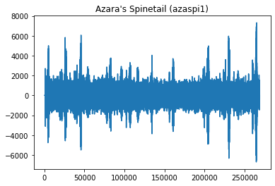
为了更好地理解数据,我们来听一听测试拆分中的随机音频文件。
注:在本笔记本的后面部分,您将对此音频运行推断以进行测试
random_audio = get_random_audio_file()
show_bird_data(random_audio)
Bird name: Azara's Spinetail
Bird code: azaspi1
训练模型
使用 Model Maker 制作音频时,必须从模型规范开始。这是基本模型,您的新模型将从中提取信息以学习新类。它还会影响如何转换数据集以符合模型规范参数,例如:采样率、通道数。
YAMNet 是在 AudioSet 数据集上训练的音频事件分类器,用于从 AudioSet 本体预测音频事件。
它的输入频率预计为 16 kHz,具有 1 个通道。
您无需自己进行任何重采样。Model Maker 会为您完成。
frame_length用于确定每个训练样本的长度。在此示例中为 EXPECTED_WAVEFORM_LENGTH * 3sframe_steps用于确定训练样本之间的距离。在本例中,第 i 个样本将在第 (i-1) 个样本后的 EXPECTED_WAVEFORM_LENGTH * 6s 处开始。
设置这些值的原因是为了绕过现实世界数据集中的一些限制。
例如,在鸟类数据集中,鸟类并不总是唱歌。它们会唱歌,休息,然后再唱歌,中间会有噪音。拥有较长的帧将有助于捕捉歌声,但将其设置得太长会减少用于训练的样本数量。
spec = audio_classifier.YamNetSpec(
    keep_yamnet_and_custom_heads=True,
    frame_step=3 * audio_classifier.YamNetSpec.EXPECTED_WAVEFORM_LENGTH,
    frame_length=6 * audio_classifier.YamNetSpec.EXPECTED_WAVEFORM_LENGTH)
INFO:tensorflow:Checkpoints are stored in /tmpfs/tmp/tmpo32sd7ga
加载数据
Model Maker 具有从文件夹加载数据并以模型规范的预期格式提供数据的 API。
训练拆分和测试拆分基于文件夹。验证数据集将被创建为训练拆分的 20%。
注:cache=True 对于提高之后的训练速度很重要,但它也需要更多的 RAM 来保存数据。对于 Birds 数据集,这不是问题,因为它只有 300MB,但如果您使用自己的数据,则必须加以注意。
train_data = audio_classifier.DataLoader.from_folder(
    spec, os.path.join(data_dir, 'train'), cache=True)
train_data, validation_data = train_data.split(0.8)
test_data = audio_classifier.DataLoader.from_folder(
    spec, os.path.join(data_dir, 'test'), cache=True)
训练模型
audio_classifier 具有 create 方法,用于创建并开始训练模型。
您可以自定义许多参数,有关更多信息,请阅读文档中的更多详细信息。
在第一次尝试中,您将使用所有默认配置并训练 100 个周期。
注:第一个周期会比所有其他周期花费更长的时间,因为此时会创建缓存。之后,每一个周期花费近 1 秒。
batch_size = 128
epochs = 100

print('Training the model')
model = audio_classifier.create(
    train_data,
    spec,
    validation_data,
    batch_size=batch_size,
    epochs=epochs)
Training the model
Model: "sequential"
_________________________________________________________________
 Layer (type)                Output Shape              Param #
=================================================================
 classification_head (Dense)  (None, 5)                5125

=================================================================
Total params: 5,125
Trainable params: 5,125
Non-trainable params: 0
_________________________________________________________________
Epoch 1/100
21/21 [==============================] - 19s 805ms/step - loss: 1.4962 - acc: 0.3230 - val_loss: 1.2149 - val_acc: 0.6796
Epoch 2/100
21/21 [==============================] - 0s 12ms/step - loss: 1.2849 - acc: 0.5033 - val_loss: 1.0718 - val_acc: 0.7058
Epoch 3/100
21/21 [==============================] - 0s 13ms/step - loss: 1.1563 - acc: 0.5890 - val_loss: 0.9997 - val_acc: 0.7662
Epoch 4/100
21/21 [==============================] - 0s 14ms/step - loss: 1.0463 - acc: 0.6567 - val_loss: 0.9374 - val_acc: 0.7902
Epoch 5/100
21/21 [==============================] - 0s 12ms/step - loss: 0.9721 - acc: 0.6817 - val_loss: 0.8918 - val_acc: 0.8084
Epoch 6/100
21/21 [==============================] - 0s 12ms/step - loss: 0.9137 - acc: 0.7067 - val_loss: 0.8554 - val_acc: 0.8164
Epoch 7/100
21/21 [==============================] - 0s 13ms/step - loss: 0.8674 - acc: 0.7205 - val_loss: 0.8218 - val_acc: 0.8255
Epoch 8/100
21/21 [==============================] - 0s 13ms/step - loss: 0.8287 - acc: 0.7297 - val_loss: 0.7996 - val_acc: 0.8084
Epoch 9/100
21/21 [==============================] - 0s 12ms/step - loss: 0.7939 - acc: 0.7436 - val_loss: 0.7799 - val_acc: 0.7959
Epoch 10/100
21/21 [==============================] - 0s 11ms/step - loss: 0.7605 - acc: 0.7559 - val_loss: 0.7614 - val_acc: 0.7868
Epoch 11/100
21/21 [==============================] - 0s 12ms/step - loss: 0.7357 - acc: 0.7670 - val_loss: 0.7482 - val_acc: 0.7731
Epoch 12/100
21/21 [==============================] - 0s 12ms/step - loss: 0.7088 - acc: 0.7701 - val_loss: 0.7333 - val_acc: 0.7651
Epoch 13/100
21/21 [==============================] - 0s 13ms/step - loss: 0.6868 - acc: 0.7778 - val_loss: 0.7232 - val_acc: 0.7594
Epoch 14/100
21/21 [==============================] - 0s 11ms/step - loss: 0.6713 - acc: 0.7905 - val_loss: 0.7127 - val_acc: 0.7537
Epoch 15/100
21/21 [==============================] - 0s 11ms/step - loss: 0.6535 - acc: 0.7839 - val_loss: 0.7071 - val_acc: 0.7423
Epoch 16/100
21/21 [==============================] - 0s 13ms/step - loss: 0.6312 - acc: 0.7974 - val_loss: 0.7011 - val_acc: 0.7343
Epoch 17/100
21/21 [==============================] - 0s 16ms/step - loss: 0.6159 - acc: 0.8147 - val_loss: 0.6943 - val_acc: 0.7286
Epoch 18/100
21/21 [==============================] - 0s 12ms/step - loss: 0.6044 - acc: 0.8151 - val_loss: 0.6923 - val_acc: 0.7218
Epoch 19/100
21/21 [==============================] - 0s 13ms/step - loss: 0.5876 - acc: 0.8193 - val_loss: 0.6850 - val_acc: 0.7184
Epoch 20/100
21/21 [==============================] - 0s 12ms/step - loss: 0.5810 - acc: 0.8224 - val_loss: 0.6806 - val_acc: 0.7184
Epoch 21/100
21/21 [==============================] - 0s 13ms/step - loss: 0.5721 - acc: 0.8181 - val_loss: 0.6784 - val_acc: 0.7206
Epoch 22/100
21/21 [==============================] - 0s 13ms/step - loss: 0.5659 - acc: 0.8205 - val_loss: 0.6742 - val_acc: 0.7229
Epoch 23/100
21/21 [==============================] - 0s 13ms/step - loss: 0.5439 - acc: 0.8366 - val_loss: 0.6706 - val_acc: 0.7206
Epoch 24/100
21/21 [==============================] - 0s 11ms/step - loss: 0.5451 - acc: 0.8331 - val_loss: 0.6727 - val_acc: 0.7161
Epoch 25/100
21/21 [==============================] - 0s 11ms/step - loss: 0.5348 - acc: 0.8354 - val_loss: 0.6688 - val_acc: 0.7195
Epoch 26/100
21/21 [==============================] - 0s 13ms/step - loss: 0.5315 - acc: 0.8354 - val_loss: 0.6693 - val_acc: 0.7172
Epoch 27/100
21/21 [==============================] - 0s 14ms/step - loss: 0.5148 - acc: 0.8435 - val_loss: 0.6681 - val_acc: 0.7161
Epoch 28/100
21/21 [==============================] - 0s 11ms/step - loss: 0.5165 - acc: 0.8385 - val_loss: 0.6661 - val_acc: 0.7172
Epoch 29/100
21/21 [==============================] - 0s 12ms/step - loss: 0.5062 - acc: 0.8420 - val_loss: 0.6618 - val_acc: 0.7172
Epoch 30/100
21/21 [==============================] - 0s 14ms/step - loss: 0.4978 - acc: 0.8389 - val_loss: 0.6630 - val_acc: 0.7149
Epoch 31/100
21/21 [==============================] - 0s 13ms/step - loss: 0.4925 - acc: 0.8512 - val_loss: 0.6670 - val_acc: 0.7115
Epoch 32/100
21/21 [==============================] - 0s 12ms/step - loss: 0.4777 - acc: 0.8516 - val_loss: 0.6626 - val_acc: 0.7149
Epoch 33/100
21/21 [==============================] - 0s 13ms/step - loss: 0.4887 - acc: 0.8458 - val_loss: 0.6643 - val_acc: 0.7138
Epoch 34/100
21/21 [==============================] - 0s 12ms/step - loss: 0.4764 - acc: 0.8535 - val_loss: 0.6627 - val_acc: 0.7138
Epoch 35/100
21/21 [==============================] - 0s 13ms/step - loss: 0.4691 - acc: 0.8531 - val_loss: 0.6661 - val_acc: 0.7115
Epoch 36/100
21/21 [==============================] - 0s 12ms/step - loss: 0.4617 - acc: 0.8639 - val_loss: 0.6625 - val_acc: 0.7115
Epoch 37/100
21/21 [==============================] - 0s 11ms/step - loss: 0.4634 - acc: 0.8551 - val_loss: 0.6595 - val_acc: 0.7149
Epoch 38/100
21/21 [==============================] - 0s 12ms/step - loss: 0.4556 - acc: 0.8581 - val_loss: 0.6635 - val_acc: 0.7092
Epoch 39/100
21/21 [==============================] - 0s 14ms/step - loss: 0.4539 - acc: 0.8562 - val_loss: 0.6586 - val_acc: 0.7138
Epoch 40/100
21/21 [==============================] - 0s 13ms/step - loss: 0.4456 - acc: 0.8651 - val_loss: 0.6580 - val_acc: 0.7138
Epoch 41/100
21/21 [==============================] - 0s 12ms/step - loss: 0.4488 - acc: 0.8581 - val_loss: 0.6625 - val_acc: 0.7138
Epoch 42/100
21/21 [==============================] - 0s 12ms/step - loss: 0.4400 - acc: 0.8662 - val_loss: 0.6663 - val_acc: 0.7104
Epoch 43/100
21/21 [==============================] - 0s 13ms/step - loss: 0.4358 - acc: 0.8693 - val_loss: 0.6630 - val_acc: 0.7092
Epoch 44/100
21/21 [==============================] - 0s 13ms/step - loss: 0.4312 - acc: 0.8685 - val_loss: 0.6606 - val_acc: 0.7115
Epoch 45/100
21/21 [==============================] - 0s 12ms/step - loss: 0.4296 - acc: 0.8716 - val_loss: 0.6667 - val_acc: 0.7058
Epoch 46/100
21/21 [==============================] - 0s 12ms/step - loss: 0.4183 - acc: 0.8697 - val_loss: 0.6571 - val_acc: 0.7138
Epoch 47/100
21/21 [==============================] - 0s 12ms/step - loss: 0.4231 - acc: 0.8727 - val_loss: 0.6603 - val_acc: 0.7138
Epoch 48/100
21/21 [==============================] - 0s 12ms/step - loss: 0.4116 - acc: 0.8727 - val_loss: 0.6650 - val_acc: 0.7115
Epoch 49/100
21/21 [==============================] - 0s 12ms/step - loss: 0.4191 - acc: 0.8720 - val_loss: 0.6620 - val_acc: 0.7115
Epoch 50/100
21/21 [==============================] - 0s 11ms/step - loss: 0.4076 - acc: 0.8793 - val_loss: 0.6676 - val_acc: 0.7070
Epoch 51/100
21/21 [==============================] - 0s 13ms/step - loss: 0.4059 - acc: 0.8762 - val_loss: 0.6679 - val_acc: 0.7058
Epoch 52/100
21/21 [==============================] - 0s 13ms/step - loss: 0.4015 - acc: 0.8758 - val_loss: 0.6654 - val_acc: 0.7070
Epoch 53/100
21/21 [==============================] - 0s 13ms/step - loss: 0.4113 - acc: 0.8670 - val_loss: 0.6664 - val_acc: 0.7058
Epoch 54/100
21/21 [==============================] - 0s 13ms/step - loss: 0.4038 - acc: 0.8735 - val_loss: 0.6765 - val_acc: 0.7058
Epoch 55/100
21/21 [==============================] - 0s 13ms/step - loss: 0.3982 - acc: 0.8800 - val_loss: 0.6735 - val_acc: 0.7058
Epoch 56/100
21/21 [==============================] - 0s 14ms/step - loss: 0.3925 - acc: 0.8735 - val_loss: 0.6768 - val_acc: 0.7047
Epoch 57/100
21/21 [==============================] - 0s 12ms/step - loss: 0.3877 - acc: 0.8777 - val_loss: 0.6714 - val_acc: 0.7058
Epoch 58/100
21/21 [==============================] - 0s 15ms/step - loss: 0.3987 - acc: 0.8747 - val_loss: 0.6818 - val_acc: 0.7035
Epoch 59/100
21/21 [==============================] - 0s 13ms/step - loss: 0.3891 - acc: 0.8762 - val_loss: 0.6782 - val_acc: 0.7058
Epoch 60/100
21/21 [==============================] - 0s 12ms/step - loss: 0.3909 - acc: 0.8716 - val_loss: 0.6776 - val_acc: 0.7058
Epoch 61/100
21/21 [==============================] - 0s 12ms/step - loss: 0.3913 - acc: 0.8827 - val_loss: 0.6830 - val_acc: 0.7035
Epoch 62/100
21/21 [==============================] - 0s 13ms/step - loss: 0.3781 - acc: 0.8889 - val_loss: 0.6849 - val_acc: 0.7024
Epoch 63/100
21/21 [==============================] - 0s 12ms/step - loss: 0.3827 - acc: 0.8724 - val_loss: 0.6837 - val_acc: 0.7035
Epoch 64/100
21/21 [==============================] - 0s 11ms/step - loss: 0.3856 - acc: 0.8762 - val_loss: 0.6901 - val_acc: 0.7024
Epoch 65/100
21/21 [==============================] - 0s 14ms/step - loss: 0.3726 - acc: 0.8827 - val_loss: 0.6908 - val_acc: 0.7024
Epoch 66/100
21/21 [==============================] - 0s 12ms/step - loss: 0.3748 - acc: 0.8762 - val_loss: 0.6839 - val_acc: 0.7047
Epoch 67/100
21/21 [==============================] - 0s 13ms/step - loss: 0.3765 - acc: 0.8866 - val_loss: 0.6855 - val_acc: 0.7035
Epoch 68/100
21/21 [==============================] - 0s 11ms/step - loss: 0.3707 - acc: 0.8897 - val_loss: 0.6868 - val_acc: 0.7058
Epoch 69/100
21/21 [==============================] - 0s 12ms/step - loss: 0.3687 - acc: 0.8835 - val_loss: 0.6927 - val_acc: 0.7024
Epoch 70/100
21/21 [==============================] - 0s 13ms/step - loss: 0.3703 - acc: 0.8824 - val_loss: 0.7016 - val_acc: 0.7047
Epoch 71/100
21/21 [==============================] - 0s 14ms/step - loss: 0.3663 - acc: 0.8843 - val_loss: 0.6936 - val_acc: 0.7047
Epoch 72/100
21/21 [==============================] - 0s 11ms/step - loss: 0.3622 - acc: 0.8858 - val_loss: 0.7080 - val_acc: 0.7035
Epoch 73/100
21/21 [==============================] - 0s 12ms/step - loss: 0.3574 - acc: 0.8912 - val_loss: 0.7048 - val_acc: 0.7047
Epoch 74/100
21/21 [==============================] - 0s 11ms/step - loss: 0.3651 - acc: 0.8816 - val_loss: 0.6980 - val_acc: 0.7024
Epoch 75/100
21/21 [==============================] - 0s 12ms/step - loss: 0.3580 - acc: 0.8900 - val_loss: 0.7062 - val_acc: 0.7035
Epoch 76/100
21/21 [==============================] - 0s 13ms/step - loss: 0.3535 - acc: 0.8877 - val_loss: 0.7155 - val_acc: 0.7035
Epoch 77/100
21/21 [==============================] - 0s 11ms/step - loss: 0.3559 - acc: 0.8904 - val_loss: 0.7099 - val_acc: 0.7070
Epoch 78/100
21/21 [==============================] - 0s 12ms/step - loss: 0.3549 - acc: 0.8870 - val_loss: 0.7055 - val_acc: 0.7070
Epoch 79/100
21/21 [==============================] - 0s 12ms/step - loss: 0.3552 - acc: 0.8862 - val_loss: 0.7049 - val_acc: 0.7058
Epoch 80/100
21/21 [==============================] - 0s 13ms/step - loss: 0.3492 - acc: 0.8847 - val_loss: 0.7150 - val_acc: 0.7058
Epoch 81/100
21/21 [==============================] - 0s 13ms/step - loss: 0.3480 - acc: 0.8916 - val_loss: 0.7075 - val_acc: 0.7058
Epoch 82/100
21/21 [==============================] - 0s 13ms/step - loss: 0.3484 - acc: 0.8912 - val_loss: 0.7089 - val_acc: 0.7058
Epoch 83/100
21/21 [==============================] - 0s 14ms/step - loss: 0.3438 - acc: 0.8939 - val_loss: 0.7106 - val_acc: 0.7070
Epoch 84/100
21/21 [==============================] - 0s 12ms/step - loss: 0.3492 - acc: 0.8866 - val_loss: 0.7172 - val_acc: 0.7081
Epoch 85/100
21/21 [==============================] - 0s 13ms/step - loss: 0.3389 - acc: 0.8923 - val_loss: 0.7150 - val_acc: 0.7081
Epoch 86/100
21/21 [==============================] - 0s 12ms/step - loss: 0.3429 - acc: 0.8858 - val_loss: 0.7230 - val_acc: 0.7081
Epoch 87/100
21/21 [==============================] - 0s 12ms/step - loss: 0.3437 - acc: 0.8904 - val_loss: 0.7251 - val_acc: 0.7081
Epoch 88/100
21/21 [==============================] - 0s 12ms/step - loss: 0.3409 - acc: 0.8931 - val_loss: 0.7194 - val_acc: 0.7092
Epoch 89/100
21/21 [==============================] - 0s 12ms/step - loss: 0.3380 - acc: 0.8850 - val_loss: 0.7271 - val_acc: 0.7081
Epoch 90/100
21/21 [==============================] - 0s 11ms/step - loss: 0.3420 - acc: 0.8881 - val_loss: 0.7180 - val_acc: 0.7070
Epoch 91/100
21/21 [==============================] - 0s 12ms/step - loss: 0.3376 - acc: 0.8954 - val_loss: 0.7335 - val_acc: 0.7081
Epoch 92/100
21/21 [==============================] - 0s 12ms/step - loss: 0.3365 - acc: 0.8870 - val_loss: 0.7347 - val_acc: 0.7058
Epoch 93/100
21/21 [==============================] - 0s 11ms/step - loss: 0.3360 - acc: 0.8923 - val_loss: 0.7172 - val_acc: 0.7092
Epoch 94/100
21/21 [==============================] - 0s 13ms/step - loss: 0.3312 - acc: 0.8908 - val_loss: 0.7342 - val_acc: 0.7081
Epoch 95/100
21/21 [==============================] - 0s 11ms/step - loss: 0.3377 - acc: 0.8904 - val_loss: 0.7291 - val_acc: 0.7092
Epoch 96/100
21/21 [==============================] - 0s 12ms/step - loss: 0.3329 - acc: 0.8966 - val_loss: 0.7362 - val_acc: 0.7070
Epoch 97/100
21/21 [==============================] - 0s 13ms/step - loss: 0.3288 - acc: 0.9008 - val_loss: 0.7318 - val_acc: 0.7081
Epoch 98/100
21/21 [==============================] - 0s 12ms/step - loss: 0.3301 - acc: 0.8897 - val_loss: 0.7399 - val_acc: 0.7081
Epoch 99/100
21/21 [==============================] - 0s 12ms/step - loss: 0.3215 - acc: 0.8973 - val_loss: 0.7356 - val_acc: 0.7092
Epoch 100/100
21/21 [==============================] - 0s 12ms/step - loss: 0.3264 - acc: 0.8958 - val_loss: 0.7370 - val_acc: 0.7081
准确率看起来很好,但重要的是对测试数据运行评估步骤,并验证您的模型是否能够在非种子数据上取得良好的结果。
print('Evaluating the model')
model.evaluate(test_data)
Evaluating the model
28/28 [==============================] - 5s 145ms/step - loss: 0.8493 - acc: 0.7692
[0.8492956757545471, 0.7692307829856873]
理解模型
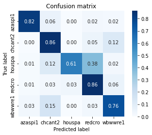
训练分类器时,查看混淆矩阵非常实用。混淆矩阵可帮助您详细了解分类器在测试数据上的性能。
Model Maker 已经为您创建了混淆矩阵。
def show_confusion_matrix(confusion, test_labels):
  """Compute confusion matrix and normalize."""
  confusion_normalized = confusion.astype("float") / confusion.sum(axis=1)
  axis_labels = test_labels
  ax = sns.heatmap(
      confusion_normalized, xticklabels=axis_labels, yticklabels=axis_labels,
      cmap='Blues', annot=True, fmt='.2f', square=True)
  plt.title("Confusion matrix")
  plt.ylabel("True label")
  plt.xlabel("Predicted label")

confusion_matrix = model.confusion_matrix(test_data)
show_confusion_matrix(confusion_matrix.numpy(), test_data.index_to_label)
1/1 [==============================] - 0s 158ms/step
1/1 [==============================] - 0s 45ms/step
1/1 [==============================] - 0s 47ms/step
1/1 [==============================] - 0s 43ms/step
1/1 [==============================] - 0s 53ms/step
1/1 [==============================] - 0s 54ms/step
1/1 [==============================] - 0s 45ms/step
1/1 [==============================] - 0s 62ms/step
1/1 [==============================] - 0s 54ms/step
1/1 [==============================] - 0s 57ms/step
1/1 [==============================] - 0s 56ms/step
1/1 [==============================] - 0s 49ms/step
1/1 [==============================] - 0s 35ms/step
1/1 [==============================] - 0s 43ms/step
1/1 [==============================] - 0s 45ms/step
1/1 [==============================] - 0s 50ms/step
1/1 [==============================] - 0s 54ms/step
1/1 [==============================] - 0s 51ms/step
1/1 [==============================] - 0s 58ms/step
1/1 [==============================] - 0s 56ms/step
1/1 [==============================] - 0s 65ms/step
1/1 [==============================] - 0s 57ms/step
1/1 [==============================] - 0s 40ms/step
1/1 [==============================] - 0s 38ms/step
1/1 [==============================] - 0s 22ms/step
1/1 [==============================] - 0s 21ms/step
1/1 [==============================] - 0s 21ms/step
1/1 [==============================] - 0s 42ms/step
测试模型 [可选]
您可以使用测试数据集中的样本音频试用该模型,以查看结果。
首先,您获得应用模型。
serving_model = model.create_serving_model()

print(f'Model\'s input shape and type: {serving_model.inputs}')
print(f'Model\'s output shape and type: {serving_model.outputs}')
Model's input shape and type: [<KerasTensor: shape=(None, 15600) dtype=float32 (created by layer 'audio')>]
Model's output shape and type: [<KerasTensor: shape=(None, 521) dtype=float32 (created by layer 'keras_layer')>, <KerasTensor: shape=(None, 5) dtype=float32 (created by layer 'sequential')>]
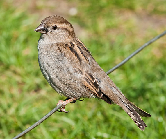
回到您之前加载的随机音频
# if you want to try another file just uncoment the line below
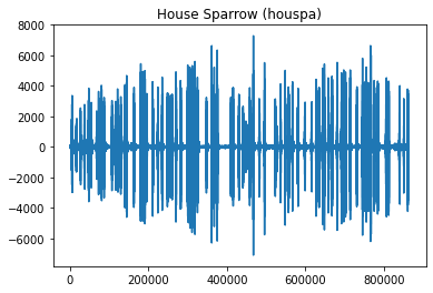
random_audio = get_random_audio_file()
show_bird_data(random_audio)
Bird name: House Sparrow
Bird code: houspa
创建的模型具有固定的输入窗口。
对于给定的音频文件,您必须将其拆分成预期大小的数据窗口。最后一个窗口可能需要用零填充。
sample_rate, audio_data = wavfile.read(random_audio, 'rb')

audio_data = np.array(audio_data) / tf.int16.max
input_size = serving_model.input_shape[1]

splitted_audio_data = tf.signal.frame(audio_data, input_size, input_size, pad_end=True, pad_value=0)

print(f'Test audio path: {random_audio}')
print(f'Original size of the audio data: {len(audio_data)}')
print(f'Number of windows for inference: {len(splitted_audio_data)}')
Test audio path: /tmpfs/src/temp/site/zh-cn/lite/models/modify/model_maker/dataset/small_birds_dataset/test/houspa/XC564822.wav
Original size of the audio data: 863968
Number of windows for inference: 56
您将循环遍历所有拆分的音频,并为每个音频应用模型。
您刚刚训练的模型有两个输出:原始 YAMNet 的输出和您刚刚训练的输出。这一点很重要,因为现实世界的环境比鸟鸣要复杂得多。您可以使用 YAMNet 的输出过滤掉不相关的音频,例如,在鸟类用例中,如果 YAMNet 没有对 Birds 或 Animals 进行分类,这可能表明您的模型的输出可能具有不相关的分类。
下面打印了两个输出,以便于理解它们之间的关系。您的模型犯错的大多数时候是当 YAMNet 的预测与您的领域不相关时(例如:鸟类)。
print(random_audio)

results = []
print('Result of the window ith:  your model class -> score,  (spec class -> score)')
for i, data in enumerate(splitted_audio_data):
  yamnet_output, inference = serving_model(data)
  results.append(inference[0].numpy())
  result_index = tf.argmax(inference[0])
  spec_result_index = tf.argmax(yamnet_output[0])
  t = spec._yamnet_labels()[spec_result_index]
  result_str = f'Result of the window {i}: ' \
  f'\t{test_data.index_to_label[result_index]} -> {inference[0][result_index].numpy():.3f}, ' \
  f'\t({spec._yamnet_labels()[spec_result_index]} -> {yamnet_output[0][spec_result_index]:.3f})'
  print(result_str)


results_np = np.array(results)
mean_results = results_np.mean(axis=0)
result_index = mean_results.argmax()
print(f'Mean result: {test_data.index_to_label[result_index]} -> {mean_results[result_index]}')
/tmpfs/src/temp/site/zh-cn/lite/models/modify/model_maker/dataset/small_birds_dataset/test/houspa/XC564822.wav
Result of the window ith:  your model class -> score,  (spec class -> score)
Result of the window 0:   houspa -> 0.900,     (Bird -> 0.916)
Result of the window 1:   houspa -> 0.860,     (Bird -> 0.812)
Result of the window 2:   houspa -> 0.576,     (Wild animals -> 0.858)
Result of the window 3:   houspa -> 0.889,     (Bird -> 0.956)
Result of the window 4:   houspa -> 0.933,     (Bird vocalization, bird call, bird song -> 0.981)
Result of the window 5:   houspa -> 0.922,     (Bird -> 0.954)
Result of the window 6:   houspa -> 0.773,     (Animal -> 0.953)
Result of the window 7:   houspa -> 0.946,     (Bird -> 0.967)
Result of the window 8:   houspa -> 0.757,     (Bird vocalization, bird call, bird song -> 0.603)
Result of the window 9:   houspa -> 0.857,     (Bird vocalization, bird call, bird song -> 0.885)
Result of the window 10:  houspa -> 0.877,     (Bird -> 0.853)
Result of the window 11:  houspa -> 0.920,     (Bird -> 0.915)
Result of the window 12:  houspa -> 0.779,     (Wild animals -> 0.947)
Result of the window 13:  houspa -> 0.786,     (Bird -> 0.852)
Result of the window 14:  houspa -> 0.616,     (Bird vocalization, bird call, bird song -> 0.928)
Result of the window 15:  houspa -> 0.994,     (Bird -> 0.999)
Result of the window 16:  houspa -> 0.891,     (Bird vocalization, bird call, bird song -> 0.967)
Result of the window 17:  houspa -> 0.969,     (Bird -> 0.953)
Result of the window 18:  houspa -> 0.712,     (Bird -> 0.898)
Result of the window 19:  redcro -> 0.574,     (Wild animals -> 0.952)
Result of the window 20:  houspa -> 0.517,     (Bird vocalization, bird call, bird song -> 0.974)
Result of the window 21:  redcro -> 0.589,     (Environmental noise -> 0.503)
Result of the window 22:  houspa -> 0.745,     (Bird -> 0.897)
Result of the window 23:  wbwwre1 -> 0.574,    (Wild animals -> 0.974)
Result of the window 24:  houspa -> 0.983,     (Bird -> 0.876)
Result of the window 25:  chcant2 -> 0.946,    (Silence -> 0.998)
Result of the window 26:  houspa -> 0.806,     (Wild animals -> 0.981)
Result of the window 27:  houspa -> 0.959,     (Bird -> 0.980)
Result of the window 28:  houspa -> 0.879,     (Bird -> 0.983)
Result of the window 29:  houspa -> 0.985,     (Bird -> 0.986)
Result of the window 30:  houspa -> 0.997,     (Bird -> 0.998)
Result of the window 31:  houspa -> 0.968,     (Bird -> 0.992)
Result of the window 32:  redcro -> 0.836,     (Environmental noise -> 0.669)
Result of the window 33:  houspa -> 0.647,     (Bird vocalization, bird call, bird song -> 0.855)
Result of the window 34:  houspa -> 0.397,     (Wild animals -> 0.927)
Result of the window 35:  houspa -> 0.952,     (Bird -> 0.955)
Result of the window 36:  houspa -> 0.819,     (Wild animals -> 0.969)
Result of the window 37:  redcro -> 0.342,     (Bird vocalization, bird call, bird song -> 0.852)
Result of the window 38:  houspa -> 0.594,     (Bird vocalization, bird call, bird song -> 0.496)
Result of the window 39:  houspa -> 0.811,     (Bird -> 0.982)
Result of the window 40:  wbwwre1 -> 0.839,    (Wild animals -> 0.986)
Result of the window 41:  houspa -> 0.985,     (Bird -> 0.973)
Result of the window 42:  wbwwre1 -> 0.616,    (Wild animals -> 0.994)
Result of the window 43:  houspa -> 0.948,     (Bird -> 0.987)
Result of the window 44:  redcro -> 0.545,     (Wild animals -> 0.902)
Result of the window 45:  houspa -> 0.974,     (Wild animals -> 0.980)
Result of the window 46:  houspa -> 0.979,     (Bird -> 0.995)
Result of the window 47:  houspa -> 0.977,     (Bird -> 0.977)
Result of the window 48:  redcro -> 0.943,     (Bird vocalization, bird call, bird song -> 0.851)
Result of the window 49:  houspa -> 0.892,     (Wild animals -> 0.985)
Result of the window 50:  houspa -> 0.984,     (Bird -> 0.980)
Result of the window 51:  houspa -> 0.980,     (Bird -> 0.969)
Result of the window 52:  houspa -> 0.968,     (Bird -> 0.977)
Result of the window 53:  houspa -> 0.920,     (Animal -> 0.996)
Result of the window 54:  houspa -> 0.809,     (Bird vocalization, bird call, bird song -> 0.708)
Result of the window 55:  houspa -> 0.634,     (Bird -> 0.962)
Mean result: houspa -> 0.7262401580810547
导出模型
最后一步是导出要在嵌入式设备或浏览器上使用的模型。
export 方法能够为您导出这两种格式。
models_path = './birds_models'
print(f'Exporing the TFLite model to {models_path}')

model.export(models_path, tflite_filename='my_birds_model.tflite')
Exporing the TFLite model to ./birds_models
INFO:tensorflow:Assets written to: /tmpfs/tmp/tmph4szi63q/assets
INFO:tensorflow:Assets written to: /tmpfs/tmp/tmph4szi63q/assets
2022-08-11 17:49:45.348759: W tensorflow/compiler/mlir/lite/python/tf_tfl_flatbuffer_helpers.cc:362] Ignored output_format.
2022-08-11 17:49:45.348875: W tensorflow/compiler/mlir/lite/python/tf_tfl_flatbuffer_helpers.cc:365] Ignored drop_control_dependency.
INFO:tensorflow:TensorFlow Lite model exported successfully: ./birds_models/my_birds_model.tflite
INFO:tensorflow:TensorFlow Lite model exported successfully: ./birds_models/my_birds_model.tflite
您还可以导出 SavedModel 版本,以便在 Python 环境中应用或使用。
model.export(models_path, export_format=[mm.ExportFormat.SAVED_MODEL, mm.ExportFormat.LABEL])
WARNING:tensorflow:Compiled the loaded model, but the compiled metrics have yet to be built. `model.compile_metrics` will be empty until you train or evaluate the model.
WARNING:tensorflow:Compiled the loaded model, but the compiled metrics have yet to be built. `model.compile_metrics` will be empty until you train or evaluate the model.
INFO:tensorflow:Assets written to: ./birds_models/saved_model/assets
INFO:tensorflow:Assets written to: ./birds_models/saved_model/assets
INFO:tensorflow:Saving labels in ./birds_models/labels.txt
INFO:tensorflow:Saving labels in ./birds_models/labels.txt
后续步骤
您成功了。
现在,您的新模型可以使用 TFLite AudioClassifier Task API 部署在移动设备上。
您还可以使用具有不同类的您自己的数据尝试相同的过程,这里是用于音频分类的 Model Maker 的文档。