TFP 版本说明笔记本 (0.11.0)

此笔记本旨在使用一些小代码段（小型化演示您可以使用 TFP 实现的内容）让 TFP 0.11.0 看起来“栩栩如生”。

在 TensorFlow.org 上查看

在 Google Colab 中运行

在 Github 上查看源代码

下载笔记本

Installs & imports

!pip3 install -U -q tensorflow==2.3.0 tensorflow_probability==0.11.0

import tensorflow as tf
import tensorflow_probability as tfp
assert '0.11' in tfp.__version__, tfp.__version__
assert '2.3' in tf.__version__, tf.__version__
tfd = tfp.distributions
tfb = tfp.bijectors
tfpk = tfp.math.psd_kernels

import matplotlib.pyplot as plt
import numpy as np
import scipy.interpolate
import IPython
import seaborn as sns

/usr/local/lib/python3.6/dist-packages/statsmodels/tools/_testing.py:19: FutureWarning: pandas.util.testing is deprecated. Use the functions in the public API at pandas.testing instead.
  import pandas.util.testing as tm

TFP 可以在 JAX 上运行

请注意，此功能已迁移至 Nightly 版本中的 tfp.substrates。

import jax
from jax.config import config
config.update('jax_enable_x64', True)

def demo_jax():
  from tensorflow_probability.python.experimental.substrates import jax as tfp
  tfd = tfp.distributions
  tfb = tfp.bijectors

  @jax.jit
  def vmap_sample(seeds):
    d = tfb.Shift(2.)(tfb.Scale(2.)(tfd.Normal(0, 1)))
    return jax.vmap(lambda seed: d.sample(seed=seed))(seeds)

  def vmap_grad(seeds, sh, sc):
    d = lambda sh, sc: tfb.Shift(sh)(tfb.Scale(sc)(tfd.Normal(0, 1)))
    return jax.vmap(
        jax.grad(lambda sh, sc, samp: d(sh, sc).log_prob(samp), 
                 argnums=(0,1,2)),
        in_axes=(None, None, 0))(sh, sc, vmap_sample(seeds))

  seed = jax.random.PRNGKey(123)
  seeds = jax.random.split(seed, 10)
  print('jit vmap sample:', vmap_sample(seeds))
  print('vmap grad:', vmap_grad(seeds, 2., 2.))

  @jax.jit
  def hmm_sample(seed):
    init, transition, obsv, sample = jax.random.split(seed, num=4)
    d = tfd.HiddenMarkovModel(
        initial_distribution=tfd.Categorical(logits=jax.random.uniform(init, [3]) + .1),
        transition_distribution=tfd.Categorical(logits=jax.random.uniform(transition, [3, 3]) + .1),
        observation_distribution=tfd.Normal(loc=jax.random.normal(obsv, [3]), scale=1.),
        num_steps=10)
    samps = d.sample(seed=sample)
    return samps, d.log_prob(samps)
  print('hmm:', hmm_sample(jax.random.PRNGKey(123)))

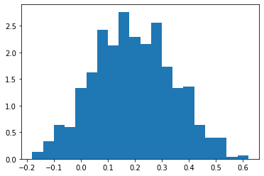
  @jax.jit
  def nuts(seed):
    return tfp.mcmc.sample_chain(
        num_results=10,
        num_burnin_steps=50,
        current_state=np.zeros([75]),
        kernel=tfp.mcmc.NoUTurnSampler(
            target_log_prob_fn=lambda x: -(x - .2)**2 / .05,
            step_size=.1),
        trace_fn=None,
        seed=seed)
  print('nuts:')
  plt.hist(nuts(seed=jax.random.PRNGKey(7)).reshape(-1), bins=20, density=True)

demo_jax()

/usr/local/lib/python3.6/dist-packages/jax/lib/xla_bridge.py:125: UserWarning: No GPU/TPU found, falling back to CPU.
  warnings.warn('No GPU/TPU found, falling back to CPU.')
jit vmap sample: [ 2.17746     2.6618252   3.427014   -0.80979496  5.87146     4.2002716
  1.2994273   1.2281269   3.5244293   4.1996603 ]
/usr/local/lib/python3.6/dist-packages/jax/numpy/lax_numpy.py:1531: FutureWarning: jax.numpy reductions won't accept lists and tuples in future versions, only scalars and ndarrays
  warnings.warn(msg, category=FutureWarning)
vmap grad: (DeviceArray([ 0.04436499,  0.1654563 ,  0.35675353, -0.70244873,
              0.96786499,  0.5500679 , -0.17514318, -0.19296828,
              0.38110733,  0.54991508], dtype=float64), DeviceArray([-0.4960635 , -0.44524843, -0.24545383,  0.48686844,
              1.37352526,  0.10514939, -0.43864973, -0.42552648,
             -0.20951441,  0.10481316], dtype=float64), DeviceArray([-0.04436499, -0.1654563 , -0.35675353,  0.7024487 ,
             -0.967865  , -0.5500679 ,  0.17514318,  0.19296828,
             -0.38110733, -0.5499151 ], dtype=float32))
hmm: (DeviceArray([-0.30260671, -0.38072154,  0.57980393, -0.30949971,
              1.22571819, -1.72733693, -1.13891736, -0.05021395,
              0.33300565, -0.31721795], dtype=float64), DeviceArray(-12.69673571, dtype=float64))
nuts:

png

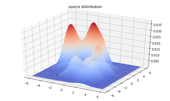
使用序贯蒙特卡洛方法的推断（试验）

nmodes = 7
loc_prior = tfd.MultivariateNormalDiag(loc=[0, 0], scale_diag=[2, 2])
mode_locs = loc_prior.sample(nmodes, seed=(0, 1))
logits_prior = tfd.Uniform()
mode_logits = logits_prior.sample(nmodes, seed=(0, 2))

make_mvn = lambda locs: tfd.MultivariateNormalDiag(
    loc=locs, scale_diag=tf.ones_like(locs))
make_mixture = lambda locs, logits: tfd.MixtureSameFamily(
    mixture_distribution=tfd.Categorical(logits=logits),
    components_distribution=make_mvn(locs))

true_dist = make_mixture(mode_locs, mode_logits)

from mpl_toolkits import mplot3d
x = np.linspace(-6, 6, 100)
y = np.linspace(-6, 6, 100)

X, Y = np.asarray(np.meshgrid(x, y), dtype=np.float32)

Z = true_dist.prob(tf.stack([X, Y], axis=-1))
fig = plt.figure(figsize=(10, 6))
ax = plt.axes(projection='3d')
ax.plot_surface(
    X, Y, Z, rstride=1, cstride=1, cmap='coolwarm', edgecolor='none')
plt.title('source distribution')
plt.show()

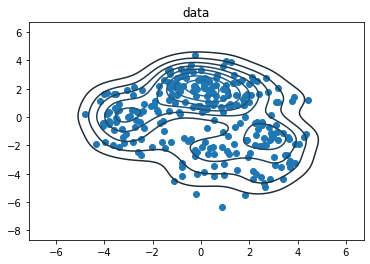
data_size = 256
samps = true_dist.sample(data_size, seed=(0, 3))
sns.kdeplot(*samps.numpy().T)
plt.scatter(*samps.numpy().T)
plt.title('data')
plt.show()

png

nparticles = 2048
seed = ()
(n_stage, final_state, final_kernel_results
  ) = tfp.experimental.mcmc.sample_sequential_monte_carlo(
      prior_log_prob_fn=lambda locs, logits: (
          tf.reduce_sum(loc_prior.log_prob(locs)) +
          tf.reduce_sum(logits_prior.log_prob(logits))),
      likelihood_log_prob_fn=lambda locs, logits: (
          tfd.Sample(make_mixture(locs, logits), data_size).log_prob(samps)),
      current_state=(loc_prior.sample([nparticles, nmodes + 2]), 
                     logits_prior.sample([nparticles, nmodes + 2])),
)

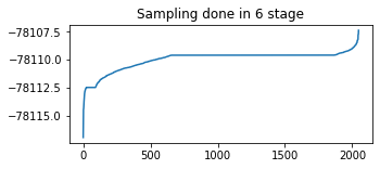
# Identify any issues with particle weight collapse.
plt.figure(figsize=(5,2))
plt.plot(tf.sort(final_kernel_results.particle_info.tempered_log_prob));
plt.title(f'Sampling done in {n_stage} stage');

png

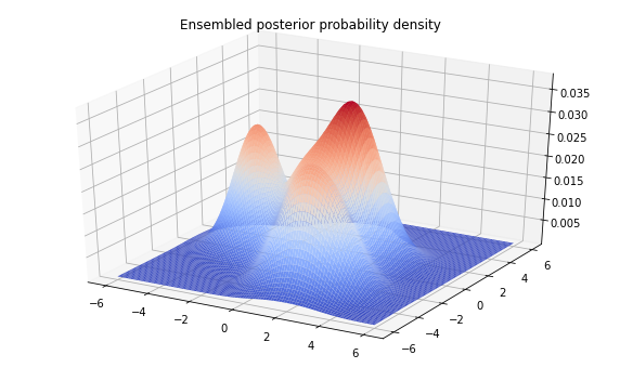
sampled_distributions = tfd.MixtureSameFamily(
    mixture_distribution=tfd.Categorical(
        logits=final_kernel_results.particle_info.tempered_log_prob),
    components_distribution=make_mixture(*final_state),
    name='ensembled_posterior')
print(sampled_distributions)
Z = sampled_distributions.prob(tf.stack([X, Y], axis=-1))
fig = plt.figure(figsize=(10, 6))
ax = plt.axes(projection='3d')
ax.plot_surface(
    X, Y, Z, rstride=1, cstride=1, cmap='coolwarm', edgecolor='none')
plt.title('Ensembled posterior probability density')
plt.show()

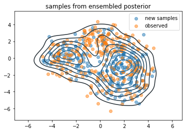
samps2 = sampled_distributions.sample(256, seed=(0, 4))
sns.kdeplot(*samps2.numpy().T)
# sns.kdeplot(*samps.numpy().T)
plt.scatter(*samps2.numpy().T, alpha=.5, label='new samples')
plt.scatter(*samps.numpy().T, alpha=.5, label='observed')
plt.legend()
plt.title('samples from ensembled posterior')
plt.show()

tfp.distributions.MixtureSameFamily("ensembled_posterior", batch_shape=[], event_shape=[2], dtype=float32)

png

球面分布：SphericalUniform（新）、PowerSpherical（新）、VonMisesFisher

`plot_spherical`

def plot_spherical(dist, nsamples):
  samples = dist.sample([nsamples], seed=123)
  probs = dist.prob(samples)
  samples = samples.numpy()
  probs = probs.numpy()
  # Show the dynamic range of the sample probabilities by re-scaling with min/max.
  minp, maxp = probs.min(), probs.max()
  ranged = np.float64(
      (probs - minp) / np.where(maxp - minp > 0, (maxp - minp), minp)) * .8 + .2

  data = list(map(list, samples))
  colors = map(plt.get_cmap('plasma'), ranged)
  colors = list(map(list, colors))

  js = """
    var scene = new THREE.Scene();
    var camera = new THREE.PerspectiveCamera( 75, 1.0, 0.1, 1000 );

    var renderer = new THREE.WebGLRenderer();
    renderer.setSize( 500, 500 );
    document.body.appendChild( renderer.domElement );

    var sphere_geom = new THREE.SphereBufferGeometry(1, 200, 200);
    var sphere_mat = new THREE.MeshBasicMaterial(
        {'opacity': 0.25, 'color': 0xFFFFFF, 'transparent': true});
    var sphere = new THREE.Mesh(sphere_geom, sphere_mat);
    sphere.position.set(0, 0, 0);
    scene.add(sphere);

    var points_data = %s;
    var points = [];
    for (var i = 0; i < points_data.length; i++) {
      points.push(new THREE.Vector3(
          points_data[i][0], points_data[i][1], points_data[i][2]));
    }

    var points_geom = new THREE.Geometry();
    points_geom.vertices = points;

    var colors_data = %s;
    var colors = [];
    for (var i = 0; i < colors_data.length; i++) {
      colors.push(new THREE.Color(
          colors_data[i][0], colors_data[i][1], colors_data[i][2]));
    }
    points_geom.colors = colors;
    var points_mat = new THREE.PointsMaterial({'size': 0.015});
    points_mat.vertexColors = THREE.VertexColors;
    var points = new THREE.Points(points_geom, points_mat);
    scene.add(points);

    camera.position.x = 0;
    camera.position.y = -2;
    camera.position.z = 2;
    camera.lookAt(new THREE.Vector3(0, 0, 0));

    controls = new THREE.TrackballControls(camera, renderer.domElement);
    controls.rotateSpeed = 1.0;
    controls.zoomSpeed = 1.2;
    controls.panSpeed = 0.8;
    controls.noZoom = false;
    controls.noPan = false;
    controls.staticMoving = false;
    controls.dynamicDampingFactor = 0.15;

    /* 
    Keep the camera pointing the same direction it was before.  However, 
    this does not generally have the same actual target as the original camera
    lookAt, only the same direction.  So when the user rotates the view it 
    might not have the expected origin of rotation. 
    */
    look_at = new THREE.Vector3(0, 0, -1);
    look_at.applyQuaternion(camera.quaternion).add(camera.position)
    controls.target = look_at;

    var LookAt = function(x, y, z) {
      camera.lookAt(new THREE.Vector3(x, y, z));
      controls.target.set(x, y, z);
    };
    LookAt(0, 0, 0);

    var animate = function () {
      requestAnimationFrame( animate );
      controls.update();
      renderer.render( scene, camera );
    };

    animate();
  """ % (repr(data), repr(colors))

  IPython.display.display_html("""
  <script type='text/javascript' src='https://ajax.googleapis.com/ajax/libs/threejs/r84/three.min.js'></script>
  <script type='text/javascript' src='https://cdn.rawgit.com/mrdoob/three.js/a1daef37/examples/js/controls/TrackballControls.js'></script>
  <script type='text/javascript'>
  %s
  </script>
  <b>Spin me!</b>
  """ % js, raw=True)

Visualizing `tfd.SphericalUniform` in 3 dimensions

nsamples = 2000 
d = tfd.SphericalUniform(dimension=3)
plot_spherical(d, nsamples)

Visualizing `tfd.PowerSpherical` in 3 dimensions

concentration = 5.0 
nsamples = 2000 
d = tfd.PowerSpherical(
    mean_direction=tf.nn.l2_normalize(np.float64([1, 1, 1]), axis=-1), 
    concentration=np.float64(concentration))
plot_spherical(d, nsamples)

Visualizing `tfd.VonMisesFisher` in 3 dimensions

concentration = 5.0 
nsamples = 2000 
vmf = tfp.distributions.VonMisesFisher(
    mean_direction=tf.nn.l2_normalize(np.float64([1, 1, 1]), axis=-1), 
    concentration=np.float64(concentration))
plot_spherical(vmf, nsamples)

新双射器

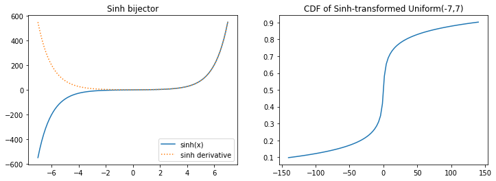
`tfb.Sinh`

plt.figure(figsize=(12, 4))
plt.subplot(121)
xs = np.linspace(-7, 7, 100)
plt.plot(xs, tfb.Sinh()(xs), label='sinh(x)')
plt.plot(xs, tf.math.exp(tfb.Sinh().forward_log_det_jacobian(xs, event_ndims=0)), ':', label='sinh derivative');
plt.legend()
plt.title('Sinh bijector')
plt.subplot(122)
xs *= 20
plt.plot(xs, tfb.Sinh()(tfd.Uniform(-7, 7)).cdf(xs))
plt.title('CDF of Sinh-transformed Uniform(-7,7)');

png

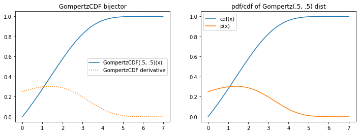
`tfb.GompertzCDF`

plt.figure(figsize=(12, 4))
plt.subplot(121)
xs = np.linspace(0, 7, 100).astype(np.float32)
b = tfb.GompertzCDF(.5, .5)
plt.plot(xs, b(xs), label='GompertzCDF(.5, .5)(x)')
plt.plot(xs, tf.math.exp(b.forward_log_det_jacobian(xs, event_ndims=0)), ':', label='GompertzCDF derivative');
plt.legend()
plt.title('GompertzCDF bijector')
plt.subplot(122)
d = tfb.Invert(b)(tfd.Uniform(0, 1))
plt.plot(xs, d.cdf(xs), label='cdf(x)')
plt.plot(xs, d.prob(xs), label='p(x)')
plt.legend()
plt.title('pdf/cdf of Gompertz(.5, .5) dist');

png

新分布

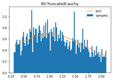
`tfd.TruncatedCauchy`

d = tfd.TruncatedCauchy(1, 1, .3, 2.1)
samples = tf.sort(d.sample(2000, seed=(0, 1)))
plt.hist(samples, bins=100, density=True, label='samples')
plt.plot(samples, d.prob(samples), label='p(x)')
plt.title('tfd.TruncatedCauchy')
plt.legend();

png

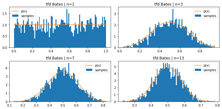
`tfd.Bates` (mean of `n` uniform samples)

plt.figure(figsize=(10, 5))
for i, n in enumerate((1, 3, 7, 13)):
  plt.subplot(221+i)
  d = tfd.Bates(total_count=n)
  samples = tf.sort(d.sample(2000, seed=(1, 2)))
  plt.hist(samples, bins=100, density=True, label='samples')
  plt.plot(samples, d.prob(samples), label='p(x)')
  plt.title(f'tfd.Bates | n={n}')
  plt.legend()
  plt.tight_layout()

png

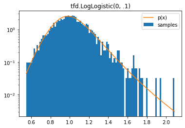
`tfd.LogLogistic`

d = tfd.LogLogistic(0, .1)
samples = tf.sort(d.sample(2000, seed=(2, 3)))
plt.hist(samples, bins=100, density=True, log=True, label='samples')
plt.plot(samples, d.prob(samples), label='p(x)')
plt.legend()
plt.title('tfd.LogLogistic(0, .1)');

png

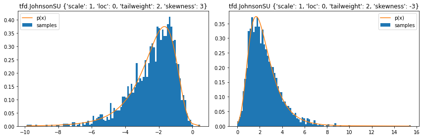
`tfd.JohnsonSU`

stats = ('loc', 'scale', 'tailweight', 'skewness')
plt.figure(figsize=(12, 4))
for i, d in enumerate([
    tfd.JohnsonSU(skewness=3, tailweight=2, loc=0, scale=1),
    tfd.JohnsonSU(skewness=-3, tailweight=2, loc=0, scale=1)]):
  plt.subplot(121+i)
  samples = tf.sort(d.sample(2000, seed=(2, 4)))
  plt.hist(samples, bins=100, density=True, label='samples')
  plt.plot(samples, d.prob(samples), label='p(x)')
  plt.legend()
  plt.title(f'tfd.JohnsonSU { {k: v for (k, v) in d.parameters.items() if k in stats} }')
  plt.tight_layout();

png

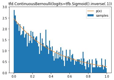
`tfd.ContinuousBernoulli`

d = tfd.ContinuousBernoulli(logits=tfb.Sigmoid().inverse(.1))
samples = tf.sort(d.sample(2000, seed=(2, 3)))
plt.hist(samples, bins=100, density=True, label='samples')
plt.plot(samples, d.prob(samples), label='p(x)')
plt.legend()
plt.title('tfd.ContinuousBernoulli(logits=tfb.Sigmoid().inverse(.1))');

png

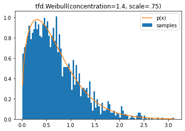
`tfd.Weibull`

d = tfd.Weibull(concentration=1.4, scale=.75)
samples = tf.sort(d.sample(2000, seed=(2, 3)))
plt.hist(samples, bins=100, density=True, label='samples')
plt.plot(samples, d.prob(samples), label='p(x)')
plt.legend()
plt.title('tfd.Weibull(concentration=1.4, scale=.75)');

png

使用 `JointDistribution*AutoBatched` 的自动向量化抽样

如果您曾经苦苦挣扎于让批次维度在联合分布中正确排列，此功能适合您。

以前编写过类似的代码？

data = tf.random.stateless_normal([7], seed=(1,2))

@tfd.JointDistributionCoroutine
def model():
  root = tfd.JointDistributionCoroutine.Root
  scale = yield root(tfd.Gamma(1, 1, name='scale'))
  yield tfd.Normal(tf.zeros_like(data), scale)

model.sample()

(<tf.Tensor: shape=(), dtype=float32, numpy=4.1253977>,
 <tf.Tensor: shape=(7,), dtype=float32, numpy=
 array([-2.814606  ,  0.81064916, -1.1025742 , -1.8684998 , -2.9547117 ,
        -0.19623983, -0.15587877], dtype=float32)>)

然后在绘制非标量样本时出现异常？

print(model.sample(1), '\n  (^^ silent badness: the second value lacks a leading (1,) shape)')
print('sampling (3,) will break:')
import traceback
try:
  model.sample(3)
except ValueError as e:
  traceback.print_exc()

(<tf.Tensor: shape=(1,), dtype=float32, numpy=array([0.15810375], dtype=float32)>, <tf.Tensor: shape=(7,), dtype=float32, numpy=
array([-0.03214252,  0.15187298, -0.08423525, -0.03807954,  0.25466064,
       -0.14433853,  0.2543037 ], dtype=float32)>) 
  (^^ silent badness: the second value lacks a leading (1,) shape)
sampling (3,) will break:
Traceback (most recent call last):
  File "/usr/local/lib/python3.6/dist-packages/tensorflow_probability/python/distributions/normal.py", line 243, in _parameter_control_dependencies
    self._batch_shape()
  File "/usr/local/lib/python3.6/dist-packages/tensorflow_probability/python/distributions/normal.py", line 176, in _batch_shape
    return tf.broadcast_static_shape(self.loc.shape, self.scale.shape)
  File "/usr/local/lib/python3.6/dist-packages/tensorflow/python/util/dispatch.py", line 201, in wrapper
    return target(*args, **kwargs)
  File "/usr/local/lib/python3.6/dist-packages/tensorflow/python/ops/array_ops.py", line 554, in broadcast_static_shape
    return common_shapes.broadcast_shape(shape_x, shape_y)
  File "/usr/local/lib/python3.6/dist-packages/tensorflow/python/framework/common_shapes.py", line 107, in broadcast_shape
    % (shape_x, shape_y))
ValueError: Incompatible shapes for broadcasting: (7,) and (3,)

During handling of the above exception, another exception occurred:

Traceback (most recent call last):
  File "<ipython-input-28-ab2fdd83415c>", line 4, in <module>
    model.sample(3)
  File "/usr/local/lib/python3.6/dist-packages/tensorflow_probability/python/distributions/distribution.py", line 939, in sample
    return self._call_sample_n(sample_shape, seed, name, **kwargs)
  File "/usr/local/lib/python3.6/dist-packages/tensorflow_probability/python/distributions/joint_distribution.py", line 532, in _call_sample_n
    **kwargs)
  File "/usr/local/lib/python3.6/dist-packages/tensorflow_probability/python/internal/distribution_util.py", line 1324, in _fn
    return fn(*args, **kwargs)
  File "/usr/local/lib/python3.6/dist-packages/tensorflow_probability/python/distributions/joint_distribution.py", line 414, in _sample_n
    **kwargs)
  File "/usr/local/lib/python3.6/dist-packages/tensorflow_probability/python/distributions/joint_distribution.py", line 451, in _call_flat_sample_distributions
    ds, xs = self._flat_sample_distributions(sample_shape, seed, value)
  File "/usr/local/lib/python3.6/dist-packages/tensorflow_probability/python/distributions/joint_distribution_coroutine.py", line 278, in _flat_sample_distributions
    d = gen.send(next_value)
  File "<ipython-input-19-d59a243cd9c8>", line 7, in model
    yield tfd.Normal(tf.zeros_like(data), scale)
  File "<decorator-gen-306>", line 2, in __init__
  File "/usr/local/lib/python3.6/dist-packages/tensorflow_probability/python/distributions/distribution.py", line 334, in wrapped_init
    default_init(self_, *args, **kwargs)
  File "/usr/local/lib/python3.6/dist-packages/tensorflow_probability/python/distributions/normal.py", line 148, in __init__
    name=name)
  File "/usr/local/lib/python3.6/dist-packages/tensorflow_probability/python/distributions/distribution.py", line 552, in __init__
    d for d in self._parameter_control_dependencies(is_init=True)
  File "/usr/local/lib/python3.6/dist-packages/tensorflow_probability/python/distributions/normal.py", line 248, in _parameter_control_dependencies
    self.loc.shape, self.scale.shape))
ValueError: Arguments `loc` and `scale` must have compatible shapes; loc.shape=(7,), scale.shape=(3,).

现在，您可以使用 `tfd.JointDistributionCoroutineAutoBatched`

编写一个“标量”抽样例程，然后绘制任意样本形状。

@tfd.JointDistributionCoroutineAutoBatched
def model_auto():
  scale = yield tfd.Gamma(1, 1, name='scale')
  yield tfd.Normal(tf.zeros_like(data), scale)

print(model_auto.sample(), '\n  (scalar sample)')
print(model_auto.sample(1), '\n  ((1,) sample)')
print(model_auto.sample(3), '\n  ((3,) sample)')

(<tf.Tensor: shape=(), dtype=float32, numpy=1.5234255>, <tf.Tensor: shape=(7,), dtype=float32, numpy=
array([-0.7177643 , -2.7825186 , -1.1250918 ,  0.57446253, -1.0755515 ,
        2.6673915 , -1.776087  ], dtype=float32)>) 
  (scalar sample)
WARNING:tensorflow:Note that RandomUniformInt inside pfor op may not give same output as inside a sequential loop.
(<tf.Tensor: shape=(1,), dtype=float32, numpy=array([0.48698178], dtype=float32)>, <tf.Tensor: shape=(1, 7), dtype=float32, numpy=
array([[ 0.44244727, -0.548889  ,  0.29392514, -0.5249126 , -0.6618264 ,
         0.06925056, -0.32040703]], dtype=float32)>) 
  ((1,) sample)
WARNING:tensorflow:Note that RandomUniformInt inside pfor op may not give same output as inside a sequential loop.
WARNING:tensorflow:Note that RandomUniformInt inside pfor op may not give same output as inside a sequential loop.
WARNING:tensorflow:Note that RandomStandardNormal inside pfor op may not give same output as inside a sequential loop.
(<tf.Tensor: shape=(3,), dtype=float32, numpy=array([0.5501703, 1.9277483, 2.7804365], dtype=float32)>, <tf.Tensor: shape=(3, 7), dtype=float32, numpy=
array([[-1.1568309 ,  0.02062727,  0.04918252, -0.08978909,  0.6446161 ,
        -0.16725235, -0.27897784],
       [-2.9246418 , -1.2733852 ,  1.0071639 , -0.4655921 , -4.1095695 ,
         0.1298227 ,  3.0307395 ],
       [-2.7411313 ,  1.6211014 , -1.600051  , -1.4009917 ,  4.081262  ,
         1.7097493 ,  2.8525631 ]], dtype=float32)>) 
  ((3,) sample)
WARNING:tensorflow:Note that RandomUniformInt inside pfor op may not give same output as inside a sequential loop.
WARNING:tensorflow:Note that RandomStandardNormal inside pfor op may not give same output as inside a sequential loop.
WARNING:tensorflow:Note that RandomStandardNormal inside pfor op may not give same output as inside a sequential loop.
(<tf.Tensor: shape=(3,), dtype=float32, numpy=array([0.5501703, 1.9277483, 2.7804365], dtype=float32)>, <tf.Tensor: shape=(3, 7), dtype=float32, numpy=
array([[-1.1568309 ,  0.02062727,  0.04918252, -0.08978909,  0.6446161 ,
        -0.16725235, -0.27897784],
       [-2.9246418 , -1.2733852 ,  1.0071639 , -0.4655921 , -4.1095695 ,
         0.1298227 ,  3.0307395 ],
       [-2.7411313 ,  1.6211014 , -1.600051  , -1.4009917 ,  4.081262  ,
         1.7097493 ,  2.8525631 ]], dtype=float32)>) 
  ((3,) sample)

可重复抽样（即使在 Eager 中也可实现）

tf.random.set_seed(123)
print('Stateful sampling:\t\t', 
      tfd.Normal(0, 1).sample(seed=234),
      'then', 
      tfd.Normal(0, 1).sample(seed=234))  

# Why are they different?
# TF samplers are stateful by default (TF maintains is a global PRNG).
# How to get reproducible results in eager mode?
tf.random.set_seed(123)
print('Stateful sampling (set_seed):\t',
      tfd.Normal(0, 1).sample(seed=234))

# And what about tf.function?
@tf.function
def sample_normal():
  return tfd.Normal(0, 1).sample(seed=234)
tf.random.set_seed(123)
print('tf.function:\t\t', sample_normal(), 'vs', sample_normal())
tf.random.set_seed(123)
print('tf.function (set_seed):\t', sample_normal())

# Using a Tensor seed (or a tuple, which TFP will convert to a tensor) induces
# TFP behavior analagous to the tf.random.stateless_* ops. This sampling 
# is fully deterministic.
print('Stateless sampling (tuple):\t\t',
      tfd.Normal(0, 1).sample(seed=(1, 23)))
print('Stateless sampling (tensor):\t\t',
      tfd.Normal(0, 1).sample(seed=tf.constant([1, 23], dtype=tf.int32)))
# Even in tf.function
@tf.function
def sample_normal():
  return tfd.Normal(0, 1).sample(seed=(1, 23))
print('Stateless sampling (tf.function):\t', sample_normal())

# And independent of global seeds.
tf.random.set_seed(321)
print('Stateless sampling (ignores set_seed):\t', sample_normal())

Stateful sampling:         tf.Tensor(0.54054874, shape=(), dtype=float32) then tf.Tensor(-1.5518123, shape=(), dtype=float32)
Stateful sampling (set_seed):  tf.Tensor(0.54054874, shape=(), dtype=float32)
tf.function:       tf.Tensor(0.54054874, shape=(), dtype=float32) vs tf.Tensor(-1.5518123, shape=(), dtype=float32)
tf.function (set_seed):    tf.Tensor(0.54054874, shape=(), dtype=float32)
Stateless sampling (tuple):        tf.Tensor(-0.36107817, shape=(), dtype=float32)
Stateless sampling (tensor):       tf.Tensor(-0.36107817, shape=(), dtype=float32)
Stateless sampling (tf.function):  tf.Tensor(-0.36107817, shape=(), dtype=float32)
Stateless sampling (ignores set_seed):     tf.Tensor(-0.36107817, shape=(), dtype=float32)

同样，`tfp.mcmc.sample_chain` 现在也接受无状态种子

这将传递到底层内核，如果这些内核给出随机建议，则必须更新这些内核才能接受 one_step 的 seed 参数。（内置内核已更新）。

kernel = tfp.mcmc.HamiltonianMonteCarlo(lambda x: -(x - .2)**2,
                                        step_size=1.,
                                        num_leapfrog_steps=2)
print_n_lines = lambda x, n: print('\n'.join(repr(x).split('\n')[:n] + ['...']))
print_n_lines(
    tfp.mcmc.sample_chain(
        num_results=5,
        num_burnin_steps=100,
        current_state=tf.zeros([3]),
        kernel=kernel,
        trace_fn=lambda state, kr: kr,
        seed=(1, 2)),
    17)
print('And again (reproducibly)...')
print_n_lines(
    tfp.mcmc.sample_chain(
        num_results=5,
        num_burnin_steps=100,
        current_state=tf.zeros([3]),
        kernel=kernel,
        trace_fn=lambda state, kr: kr,
        seed=(1, 2)),
    17)

StatesAndTrace(
  all_states=<tf.Tensor: shape=(5, 3), dtype=float32, numpy=
    array([[ 4.0000078e-01,  3.9999962e-01,  3.9999855e-01],
           [-8.3446503e-07,  3.5762787e-07,  1.5497208e-06],
           [ 4.0000081e-01,  3.9999965e-01,  3.9999846e-01],
           [-8.3446503e-07,  4.7683716e-07,  1.5497208e-06],
           [ 4.0000087e-01,  3.9999962e-01,  3.9999843e-01]], dtype=float32)>,
  trace=MetropolisHastingsKernelResults(
      accepted_results=UncalibratedHamiltonianMonteCarloKernelResults(
          log_acceptance_correction=<tf.Tensor: shape=(5, 3), dtype=float32, numpy=
            array([[ 0.0000000e+00, -2.9802322e-08,  0.0000000e+00],
                   [ 5.9604645e-08,  1.1175871e-08,  1.1920929e-07],
                   [-2.9802322e-08, -2.7939677e-09,  2.7939677e-09],
                   [ 0.0000000e+00,  0.0000000e+00, -5.9604645e-08],
                   [ 1.4901161e-08, -1.7881393e-07,  0.0000000e+00]], dtype=float32)>,
          target_log_prob=<tf.Tensor: shape=(5, 3), dtype=float32, numpy=
            array([[-0.04000031, -0.03999985, -0.03999942],
...
And again (reproducibly)...
StatesAndTrace(
  all_states=<tf.Tensor: shape=(5, 3), dtype=float32, numpy=
    array([[ 4.0000078e-01,  3.9999962e-01,  3.9999855e-01],
           [-8.3446503e-07,  3.5762787e-07,  1.5497208e-06],
           [ 4.0000081e-01,  3.9999965e-01,  3.9999846e-01],
           [-8.3446503e-07,  4.7683716e-07,  1.5497208e-06],
           [ 4.0000087e-01,  3.9999962e-01,  3.9999843e-01]], dtype=float32)>,
  trace=MetropolisHastingsKernelResults(
      accepted_results=UncalibratedHamiltonianMonteCarloKernelResults(
          log_acceptance_correction=<tf.Tensor: shape=(5, 3), dtype=float32, numpy=
            array([[ 0.0000000e+00, -2.9802322e-08,  0.0000000e+00],
                   [ 5.9604645e-08,  1.1175871e-08,  1.1920929e-07],
                   [-2.9802322e-08, -2.7939677e-09,  2.7939677e-09],
                   [ 0.0000000e+00,  0.0000000e+00, -5.9604645e-08],
                   [ 1.4901161e-08, -1.7881393e-07,  0.0000000e+00]], dtype=float32)>,
          target_log_prob=<tf.Tensor: shape=(5, 3), dtype=float32, numpy=
            array([[-0.04000031, -0.03999985, -0.03999942],
...

完美打印 MCMC 内核结果

tfp.mcmc.RandomWalkMetropolis(tfd.Uniform(0, 10).log_prob).bootstrap_results(1.)

MetropolisHastingsKernelResults(
  accepted_results=UncalibratedRandomWalkResults(
      log_acceptance_correction=<tf.Tensor: shape=(), dtype=float32, numpy=0.0>,
      target_log_prob=<tf.Tensor: shape=(), dtype=float32, numpy=-2.3025851>,
      seed=[]
    ),
  is_accepted=<tf.Tensor: shape=(), dtype=bool, numpy=True>,
  log_accept_ratio=<tf.Tensor: shape=(), dtype=float32, numpy=0.0>,
  proposed_state=1.0,
  proposed_results=UncalibratedRandomWalkResults(
      log_acceptance_correction=<tf.Tensor: shape=(), dtype=float32, numpy=0.0>,
      target_log_prob=<tf.Tensor: shape=(), dtype=float32, numpy=-2.3025851>,
      seed=<tf.Tensor: shape=(2,), dtype=int32, numpy=array([0, 0], dtype=int32)>
    ),
  extra=[],
  seed=<tf.Tensor: shape=(2,), dtype=int32, numpy=array([0, 0], dtype=int32)>
)

CompositeTensor（实验性）

减少对 tf.function 的跟踪。从 tf.function 返回分布。

@tf.function
def get_mean(d):
  return d.mean()

print(get_mean(tfp.experimental.as_composite(tfd.BetaBinomial(100., 2., 7.))))

@tf.function
def returns_dist(logits):
  return tfp.experimental.as_composite(tfd.Binomial(10., logits=logits))

print(returns_dist(tf.constant(0.)),
      returns_dist(tf.constant(0.)).sample(seed=(2, 3)))

tf.Tensor(22.222221, shape=(), dtype=float32)
tfp.distributions.BinomialCT("Binomial", batch_shape=[], event_shape=[], dtype=float32) tf.Tensor(5.0, shape=(), dtype=float32)

您是否知道批次切片分布

def demo_batch_slice():
  d = tfd.Normal(
      loc=tf.random.stateless_normal([100, 20, 3], seed=(1,2)),
      scale=1.)
  print(d, '\n  (original dist)')
  print(d[0], '\n  (0th element of the first batch dimension)')
  print(d[::2, ..., 1], '\n  (every other element of first dim  x  middle element of final dim)\n')

  d = tfd.Dirichlet(
      concentration=tf.random.stateless_uniform([100, 20, 3, 7], seed=(1,2)))
  print(d, '\n  (original dist)')
  print(d[:, 0], '\n  (0th element of the second dimension)')
  print(d[::2, ..., 1], '\n  (every other element of first dim  x  middle element of final dim)')
demo_batch_slice()

tfp.distributions.Normal("Normal", batch_shape=[100, 20, 3], event_shape=[], dtype=float32) 
  (original dist)
tfp.distributions.Normal("Normal", batch_shape=[20, 3], event_shape=[], dtype=float32) 
  (0th element of the first batch dimension)
tfp.distributions.Normal("Normal", batch_shape=[50, 20], event_shape=[], dtype=float32) 
  (every other element of first dim  x  middle element of final dim)

tfp.distributions.Dirichlet("Dirichlet", batch_shape=[100, 20, 3], event_shape=[7], dtype=float32) 
  (original dist)
tfp.distributions.Dirichlet("Dirichlet", batch_shape=[100, 3], event_shape=[7], dtype=float32) 
  (0th element of the second dimension)
tfp.distributions.Dirichlet("Dirichlet", batch_shape=[50, 20], event_shape=[7], dtype=float32) 
  (every other element of first dim  x  middle element of final dim)

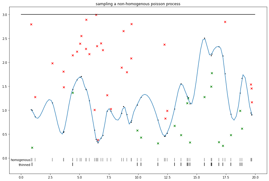
随机新奇事物：对 S 形 Cox（非均质泊松）过程抽样

我们可以使用 Adams 等人提议的细化程序。

请注意，类似的细化方式与不可逆 MCMC（例如，锯齿和弹性粒子抽样器）的一些方式相关，其中，强度上限可用于对非均质事件抽样。

def sigmoidal_cox_process():
  V = 20.
  lam0 = 3.
  n_homog = tfd.Poisson(V * lam0).sample(seed=(0, 1))
  homog_locs = tf.sort(tfd.Uniform(0., V).sample(n_homog, seed=(0, 2)))
  homog_intensities = tfd.GaussianProcess(
      tfpk.MaternThreeHalves(), 
      index_points=homog_locs[:, tf.newaxis]).sample(seed=(0, 3))

  plt.figure(figsize=(15,10))
  plt.title('sampling a non-homogenous poisson process')
  plt.hlines(lam0, xmin=0., xmax=V)

  sigm_int = tf.math.sigmoid(homog_intensities) * lam0

  sp = scipy.interpolate.make_interp_spline(homog_locs, sigm_int)
  xs = np.linspace(homog_locs[0], homog_locs[-1], 100)
  ys = scipy.interpolate.splev(xs, sp)
  plt.plot(xs, ys)

  plt.scatter(homog_locs, sigm_int, s=5., c='black')

  unif = tfd.Uniform(0, lam0).sample(n_homog)
  plt.scatter(homog_locs, tf.where(unif < sigm_int, np.nan, unif), c='r', marker='x')
  plt.scatter(homog_locs, tf.where(unif > sigm_int, np.nan, unif), c='g', marker='x')

  plt.vlines(homog_locs, 0, -.07, colors='gray', )
  plt.text(.8, -.06, 'homogenous', dict(fontsize='medium'), horizontalalignment='right')

  nonhomog_locs = tf.gather(homog_locs, tf.where(unif < sigm_int))
  plt.vlines(nonhomog_locs, -.1, -.17, colors='black')
  plt.text(.8, -.16, 'thinned', dict(fontsize='medium'), horizontalalignment='right')
  plt.show()

sigmoidal_cox_process()

png

您是否知道 GP 的批次

高斯过程是函数的分布。在此，我们将通过内核和一组索引点进行参数化，并展现一些批处理行为。

（TFP 也支持 GP 回归模型，在该模型中，观测的索引点的观测值可确定一组索引点的函数的后验分布，请参阅 tfd.GaussianProcessRegressionModel。）

from mpl_toolkits import mplot3d
x = np.linspace(-6, 6, 9)
y = np.linspace(-6, 6, 9)

X, Y = np.asarray(np.meshgrid(x, y), dtype=np.float32)

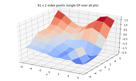
print('We can set up a single GP over many examples of 2d feature')
gp = tfd.GaussianProcess(
    tfpk.ExponentiatedQuadratic(length_scale=3., feature_ndims=1),
    index_points=tf.reshape(tf.stack([X, Y], axis=-1), (-1, 2)),
    jitter=1e-3)
print(gp)
Z = tf.reshape(gp.sample(seed=(0,3)), X.shape)
fig = plt.figure(figsize=(10, 6))
ax = plt.axes(projection='3d')
ax.plot_surface(
    X, Y, Z, rstride=1, cstride=1, cmap='coolwarm', edgecolor='none');
ax.set_xlabel('x');ax.set_ylabel('y');
ax.set_title('81 x 2 index points (single GP over all pts)')
plt.show()

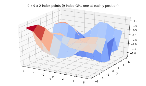
print('We can have a batch of independent GPs with their own sets of index points.')
batch_gp = tfd.GaussianProcess(
    tfpk.ExponentiatedQuadratic(length_scale=3., feature_ndims=1),
    index_points=tf.stack([X, Y], axis=-1),
    jitter=1e-3)
print(batch_gp)
Z_batch = batch_gp.sample(seed=(5,7))
fig = plt.figure(figsize=(10, 6))
ax = plt.axes(projection='3d')
ax.plot_surface(
    X, Y, Z_batch, rstride=1, cstride=1, cmap='coolwarm', edgecolor='none');
ax.set_xlabel('x');ax.set_ylabel('y');
ax.set_title('9 x 9 x 2 index points (9 indep GPs, one at each y position)');
plt.show()

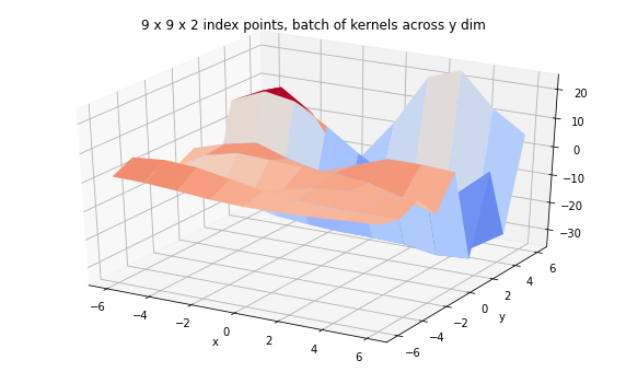
print('We can also have a corresponding batch of kernels.')
kernel = tfpk.ExponentiatedQuadratic(length_scale=3.,
                                     amplitude=tf.linspace(1., 20., 9),
                                     feature_ndims=1)
print(kernel)
batch_gp_kernel = tfd.GaussianProcess(
    kernel,
    index_points=tf.stack([X, Y], axis=-1),
    jitter=1e-3)
print(batch_gp_kernel)
Z_batch_kernel = batch_gp_kernel.sample(seed=(5,7))

fig = plt.figure(figsize=(10, 6))
ax = plt.axes(projection='3d')
ax.plot_surface(
    X, Y, Z_batch_kernel, rstride=1, cstride=1, cmap='coolwarm', edgecolor='none');
ax.set_xlabel('x');ax.set_ylabel('y');
ax.set_title('9 x 9 x 2 index points, batch of kernels across y dim');

We can set up a single GP over many examples of 2d feature
tfp.distributions.GaussianProcess("GaussianProcess", batch_shape=[], event_shape=[81], dtype=float32)

png

We can also have a corresponding batch of kernels.
tfp.math.psd_kernels.ExponentiatedQuadratic("ExponentiatedQuadratic", batch_shape=(9,), feature_ndims=1, dtype=float32)
tfp.distributions.GaussianProcess("GaussianProcess", batch_shape=[9], event_shape=[9], dtype=float32)

png

We can also have a corresponding batch of kernels.
tfp.math.psd_kernels.ExponentiatedQuadratic("ExponentiatedQuadratic", batch_shape=(9,), feature_ndims=1, dtype=float32)
tfp.distributions.GaussianProcess("GaussianProcess", batch_shape=[9], event_shape=[9], dtype=float32)

png

TFP 版本说明笔记本 (0.11.0)

Installs & imports

TFP 可以在 JAX 上运行

使用序贯蒙特卡洛方法的推断（试验）

球面分布：SphericalUniform（新）、PowerSpherical（新）、VonMisesFisher

plot_spherical

Visualizing tfd.SphericalUniform in 3 dimensions

Visualizing tfd.PowerSpherical in 3 dimensions

Visualizing tfd.VonMisesFisher in 3 dimensions

新双射器

tfb.Sinh

tfb.GompertzCDF

新分布

tfd.TruncatedCauchy

tfd.Bates (mean of n uniform samples)

tfd.LogLogistic

tfd.JohnsonSU

tfd.ContinuousBernoulli

tfd.Weibull

使用 JointDistribution*AutoBatched 的自动向量化抽样