Aşağıda XlaBuilder arayüzünde tanımlanan işlemlerin anlamı açıklanmaktadır. Genellikle bu işlemler bire bir işlemleri xla_data.proto içindeki RPC arayüzünde tanımlanan işlemlerle eşler.
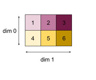
Ölçüyle ilgili bir not: XLA'nın genelleştirilmiş veri türünün ele aldığı, bazı tek tip türlerdeki (32 bitlik kayan nokta gibi) öğeleri içeren N boyutlu bir dizidir. Belgelendirmede dizi, rastgele boyutlu bir diziyi göstermek için kullanılır. Kolaylık sağlaması açısından, özel durumların daha spesifik ve tanıdık adları vardır. Örneğin, vektör 1 boyutlu bir dizidir ve matris, 2 boyutlu bir dizidir.
AfterAll
Ayrıca bkz.
XlaBuilder::AfterAll.
AfterAll, çeşitli sayıda jeton alır ve tek bir jeton oluşturur. Jetonlar, sıralamayı zorunlu kılmak için yan etkisi olan işlemler arasında işlenebilir temel türlerdir. AfterAll, belirli bir işlemden sonra işlem sipariş etmek için jetonların birleştirilmesi olarak kullanılabilir.
AfterAll(operands)
| Bağımsız değişkenler | Tür | Anlambilim |
|---|---|---|
operands |
XlaOp |
değişken sayıda jeton |
AllGather
Ayrıca bkz.
XlaBuilder::AllGather.
Kopyalar arasında birleştirme gerçekleştirir.
AllGather(operand, all_gather_dim, shard_count, replica_group_ids,
channel_id)
| Bağımsız değişkenler | Tür | Anlambilim |
|---|---|---|
operand
|
XlaOp
|
Çoğaltmalar arasında birleştirilecek dizi |
all_gather_dim |
int64 |
Birleştirme boyutu |
replica_groups
|
int64 vektörünün
vektörü |
Aralarında birleştirmenin gerçekleştirildiği gruplar |
channel_id
|
isteğe bağlı int64
|
Modüller arası iletişim için isteğe bağlı kanal kimliği |
replica_groups, birleştirme işleminin gerçekleştirildiği replika gruplarının listesidir (geçerli replikanın replika kimliğiReplicaIdkullanılarak alınabilir). Her gruptaki replikaların sırası, girişlerinin sonuçtaki sıralarını belirler.replica_groupsya boş olmalı (bu durumda tüm replikalar tek bir gruba ait olmalı ve0ileN - 1arasında sıralanmıştır) ya da replika sayısıyla aynı sayıda öğe içermelidir. Örneğinreplica_groups = {0, 2}, {1, 3},0ile2replikaları ile1ve3replikaları arasında birleştirme işlemi gerçekleştirir.shard_count, her bir replika grubunun boyutudur.replica_groupsdeğerinin boş olduğu durumlarda buna ihtiyacımız vardır.channel_id, modüller arası iletişim için kullanılır: Yalnızca aynıchannel_iddeğerine sahipall-gatherişlemleri birbiriyle iletişim kurabilir.
Çıkış şekli, shard_count kat daha büyük hale getirilmiş all_gather_dim ile giriş şeklidir. Örneğin, iki replika varsa ve işlenen iki replikada sırasıyla [1.0, 2.5] ve [3.0, 5.25] değerine sahipse all_gather_dim'nin 0 olduğu bu işlemden elde edilen çıkış değeri her iki replikada da [1.0, 2.5, 3.0,
5.25] olur.
AllReduce
Ayrıca bkz.
XlaBuilder::AllReduce.
Replikalar arasında özel bir hesaplama yapar.
AllReduce(operand, computation, replica_group_ids, channel_id)
| Bağımsız değişkenler | Tür | Anlambilim |
|---|---|---|
operand
|
XlaOp
|
Replikalar genelinde azaltılacak dizi veya boş olmayan diziler |
computation |
XlaComputation |
Azaltma hesaplaması |
replica_groups
|
int64 vektörünün
vektörü |
Aralarında azaltmaların uygulandığı gruplar |
channel_id
|
isteğe bağlı int64
|
Modüller arası iletişim için isteğe bağlı kanal kimliği |
operandbir dizi unsur olduğunda, devir işlemi söz konusu değin her bir öğesi için tümüyle indirgeme işlemi gerçekleştirilir.replica_groups, azaltmanın gerçekleştirildiği replika gruplarının listesidir (geçerli replikanın replika kimliğiReplicaIdkullanılarak alınabilir).replica_groupsboş olmalı (tüm replikalar tek bir gruba ait olduğunda) ya da replika sayısı ile aynı sayıda öğe içermelidir. Örneğinreplica_groups = {0, 2}, {1, 3},0ile2replikaları ile1ve3replikaları arasında azaltma gerçekleştirir.channel_id, modüller arası iletişim için kullanılır: Yalnızca aynıchannel_iddeğerine sahipall-reduceişlemleri birbiriyle iletişim kurabilir.
Çıkış şekli giriş şekliyle aynıdır. Örneğin, iki replika varsa ve işlenen, iki replikada sırasıyla [1.0, 2.5] ve [3.0, 5.25] değerlerine sahipse bu işlem ve toplama hesaplamasından elde edilen çıkış değeri her iki replikada da [4.0, 7.75] olur. Giriş de bir unsur ise çıkış da bir unsurdur.
AllReduce sonucunu hesaplamak için her replikadan bir giriş olması gerekir. Bu nedenle, bir replika AllReduce düğümünü diğerinden daha fazla kez yürütürse eski replika sonsuza kadar bekler. Replikaların tümü aynı programı çalıştırdığından bunu yapmanın pek çok yolu yoktur ancak bir süre döngüsünün koşulu feed'deki verilere bağlı olduğunda ve beslenen veriler, zaman döngüsünün bir replikada diğerinden daha fazla iterasyon yapmasına neden olduğunda mümkündür.
AllToAll
Ayrıca bkz.
XlaBuilder::AllToAll.
AllToAll, tüm çekirdeklerden tüm çekirdeklere veri gönderen toplu bir işlemdir. İki aşamadan oluşur:
- Dağılım aşaması. Her çekirdekte işlenen
split_count,split_dimensionsboyunca bulunan bloğa bölünür ve bloklar tüm çekirdeklere yayılır.Ör. i'ninci çekirdeğe gönderilir. - Toplama aşaması. Her çekirdek,
concat_dimensionboyunca alınan blokları birleştirir.
Katılan çekirdekler şu şekilde yapılandırılabilir:
replica_groups: Her ReplicaGroup, hesaplamada yer alan replika kimliklerinin listesini içerir (mevcut kopyanın replika kimliğiReplicaIdkullanılarak alınabilir). AllToAll, belirtilen sıradaki alt gruplar içinde uygulanır. Örneğinreplica_groups = { {1,2,3}, {4,5,0} }, bir AllToAll'un{1, 2, 3}replikaları içinde uygulanacağı ve toplama aşamasında alınan blokların aynı sırada 1, 2, 3 ile birleştirileceği anlamına gelir. Ardından 4, 5, 0 replikalarına başka bir AllToAll uygulanır ve birleştirme sırası da 4, 5, 0 olur.replica_groupsboşsa tüm replikalar, görünüm sıralamasında bir gruba ait olur.
Ön koşullar:
split_dimensionüzerindeki işlenenin boyut boyutusplit_countile bölünebilir.- İşlem görenin şekli tuple değil.
AllToAll(operand, split_dimension, concat_dimension, split_count,
replica_groups)
| Bağımsız değişkenler | Tür | Anlambilim |
|---|---|---|
operand |
XlaOp |
n boyutlu giriş dizisi |
split_dimension
|
int64
|
[0,
n)
aralığında işlenenin bölündüğü boyutu belirten bir değer |
concat_dimension
|
int64
|
[0,
n)
aralığında, bölme bloklarının birleştirildiği boyutu adlandıran bir değer |
split_count
|
int64
|
Bu işleme katılan çekirdeklerin sayısı. replica_groups boşsa bu, replika sayısı olmalıdır. Aksi takdirde, her bir gruptaki replika sayısına eşit olmalıdır. |
replica_groups
|
ReplicaGroup vektör
|
Her grupta bir replika kimlikleri listesi bulunur. |
Aşağıda bir Alltoall örneği gösterilmektedir.
XlaBuilder b("alltoall");
auto x = Parameter(&b, 0, ShapeUtil::MakeShape(F32, {4, 16}), "x");
AllToAll(x, /*split_dimension=*/1, /*concat_dimension=*/0, /*split_count=*/4);
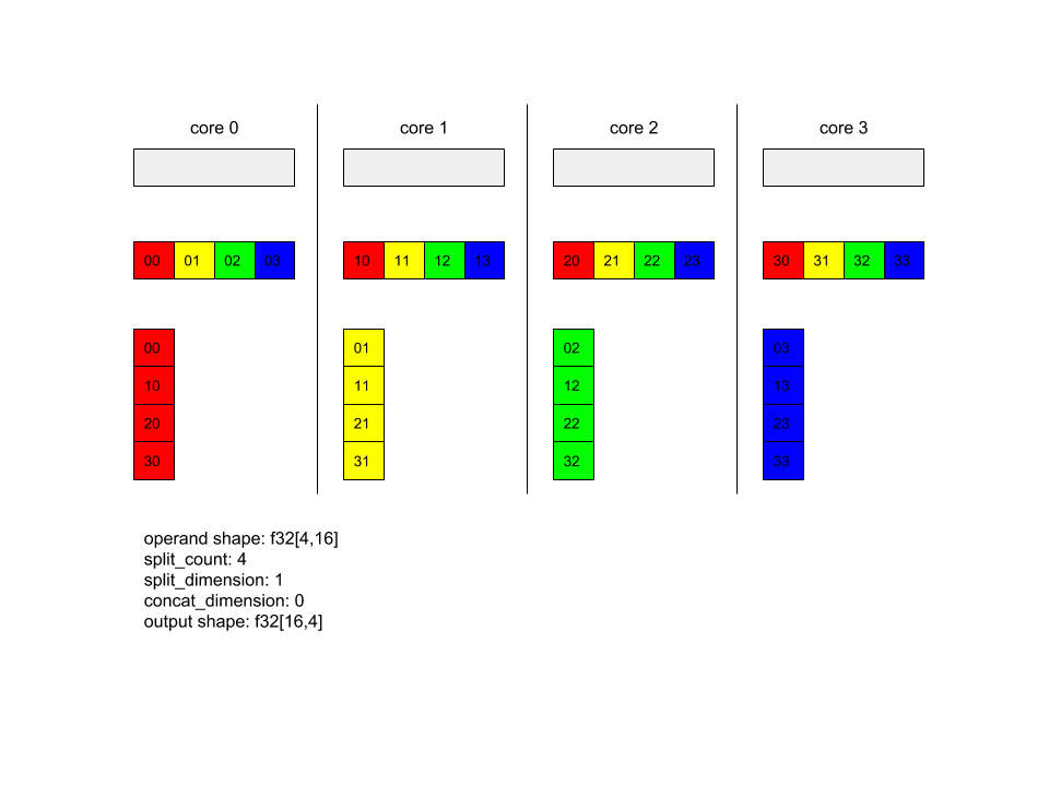
Bu örnekte, Alltoall katılımı 4 çekirdektir. Her çekirdekte işlenen, 0 boyutu boyunca 4 bölüme ayrılmıştır. Böylece her parça f32[4,4] şekline sahiptir. 4 bölüm tüm çekirdeklere yayılır. Daha sonra her çekirdek, alınan parçaları 1. boyut boyunca, çekirdek 0-4 arasında bir araya getirir. Her bir çekirdekteki çıkışın şekli f32[16,4] olur.
BatchNormGrad
Algoritmanın ayrıntılı açıklaması için XlaBuilder::BatchNormGrad ve orijinal toplu normalleştirme makalesine de bakın.
Toplu normun gradyanlarını hesaplar.
BatchNormGrad(operand, scale, mean, variance, grad_output, epsilon, feature_index)
| Bağımsız değişkenler | Tür | Anlambilim |
|---|---|---|
operand |
XlaOp |
Normalleştirilecek n boyutlu dizi (x) |
scale |
XlaOp |
1 boyutsal dizi (\(\gamma\)) |
mean |
XlaOp |
1 boyutsal dizi (\(\mu\)) |
variance |
XlaOp |
1 boyutsal dizi (\(\sigma^2\)) |
grad_output |
XlaOp |
Renk geçişleri BatchNormTraining (\(\nabla y\)) sürümüne geçirildi |
epsilon |
float |
Epsilon değeri (\(\epsilon\)) |
feature_index |
int64 |
operand içindeki özellik boyutu dizini |
Özellik boyutundaki her bir özellik için (feature_index, operand öğesindeki özellik boyutunun dizinidir) işlem, gradyanları diğer tüm boyutlarda operand, offset ve scale'a göre hesaplar. feature_index, operand içindeki özellik boyutu için geçerli bir dizin olmalıdır.
Bu üç renk geçiş, aşağıdaki formüllerle tanımlanır (operand şeklinde 4 boyutlu bir dizinin ve l özellik boyutu dizinine, m grup boyutuna ve w ile h mekansal boyutlarına sahip olduğu varsayılır):
\[ \begin{split} c_l&= \frac{1}{mwh}\sum_{i=1}^m\sum_{j=1}^w\sum_{k=1}^h \left( \nabla y_{ijkl} \frac{x_{ijkl} - \mu_l}{\sigma^2_l+\epsilon} \right) \\\\ d_l&= \frac{1}{mwh}\sum_{i=1}^m\sum_{j=1}^w\sum_{k=1}^h \nabla y_{ijkl} \\\\ \nabla x_{ijkl} &= \frac{\gamma_{l} }{\sqrt{\sigma^2_{l}+\epsilon} } \left( \nabla y_{ijkl} - d_l - c_l (x_{ijkl} - \mu_{l}) \right) \\\\ \nabla \gamma_l &= \sum_{i=1}^m\sum_{j=1}^w\sum_{k=1}^h \left( \nabla y_{ijkl} \frac{x_{ijkl} - \mu_l}{\sqrt{\sigma^2_{l}+\epsilon} } \right) \\\\\ \nabla \beta_l &= \sum_{i=1}^m\sum_{j=1}^w\sum_{k=1}^h \nabla y_{ijkl} \end{split} \]
mean ve variance girdileri, toplu ve uzamsal boyutlardaki an değerlerini temsil eder.
Çıkış türü, üç herkese açık kullanıcı adından oluşur:
| Çıkışlar | Tür | Anlambilim |
|---|---|---|
grad_operand
|
XlaOp
|
girişe göre gradyanı: operand ($\nabla
x$) |
grad_scale
|
XlaOp
|
girişe göre gradyanı: scale ($\nabla
\gamma$) |
grad_offset
|
XlaOp
|
girişe göre gradyan offset($\nabla
\beta$) |
BatchNormInference
Algoritmanın ayrıntılı açıklaması için XlaBuilder::BatchNormInference ve orijinal toplu normalleştirme makalesine de bakın.
Bir diziyi toplu ve uzamsal boyutlarda normalleştirir.
BatchNormInference(operand, scale, offset, mean, variance, epsilon, feature_index)
| Bağımsız değişkenler | Tür | Anlambilim |
|---|---|---|
operand |
XlaOp |
Normalleştirilecek n boyutlu dizi |
scale |
XlaOp |
1 boyutlu dizi |
offset |
XlaOp |
1 boyutlu dizi |
mean |
XlaOp |
1 boyutlu dizi |
variance |
XlaOp |
1 boyutlu dizi |
epsilon |
float |
Epsilon değeri |
feature_index |
int64 |
operand içindeki özellik boyutu dizini |
Özellik boyutundaki her bir özellik (feature_index, operand özelliğindeki özellik boyutunun dizinidir) için işlem, diğer tüm boyutlarda ortalama ve varyansı hesaplar ve operand öğesindeki her bir öğeyi normalleştirmek için ortalama ve varyansı kullanır. feature_index, operand içindeki özellik boyutu için geçerli bir dizin olmalıdır.
BatchNormInference, her grup için mean ve variance hesaplamadan BatchNormTraining çağırmaya eş değerdir. Bunun yerine tahmini değerler olarak mean ve variance girdilerini kullanır. Bu işlemin amacı, çıkarımdaki gecikmeyi azaltmaktır. Bu nedenle adı BatchNormInference.
Çıkış, operand girişiyle aynı şekle sahip n boyutlu, normalleştirilmiş bir dizidir.
BatchNormTraining
Algoritmanın ayrıntılı açıklaması için XlaBuilder::BatchNormTraining ve the original batch normalization paper bölümlerine de göz atın.
Bir diziyi toplu ve uzamsal boyutlarda normalleştirir.
BatchNormTraining(operand, scale, offset, epsilon, feature_index)
| Bağımsız değişkenler | Tür | Anlambilim |
|---|---|---|
operand |
XlaOp |
Normalleştirilecek n boyutlu dizi (x) |
scale |
XlaOp |
1 boyutsal dizi (\(\gamma\)) |
offset |
XlaOp |
1 boyutsal dizi (\(\beta\)) |
epsilon |
float |
Epsilon değeri (\(\epsilon\)) |
feature_index |
int64 |
operand içindeki özellik boyutu dizini |
Özellik boyutundaki her bir özellik (feature_index, operand özelliğindeki özellik boyutunun dizinidir) için işlem, diğer tüm boyutlarda ortalama ve varyansı hesaplar ve operand öğesindeki her bir öğeyi normalleştirmek için ortalama ve varyansı kullanır. feature_index, operand içindeki özellik boyutu için geçerli bir dizin olmalıdır.
Algoritma, operand \(x\) konumunda konumsal boyutların boyutu olarak w ve h içeren m öğeleri içeren her bir grup için aşağıdaki gibi gider (operand öğesinin 4 boyutlu bir dizi olduğu varsayılır):
Özellik boyutundaki her özellik
liçin toplu ortalamayı \(\mu_l\) hesaplar: \(\mu_l=\frac{1}{mwh}\sum_{i=1}^m\sum_{j=1}^w\sum_{k=1}^h x_{ijkl}\)Toplu varyansı hesaplar \(\sigma^2_l\): $\sigma^2l=\frac{1}{mwh}\sum{i=1}^m\sum{j=1}^w\sum{k=1}^h (x_{ijkl} - \mu_l)^2$
Normalleştirir, ölçeklendirir ve değiştirir: \(y_{ijkl}=\frac{\gamma_l(x_{ijkl}-\mu_l)}{\sqrt[2]{\sigma^2_l+\epsilon} }+\beta_l\)
Sıfıra bölme hatalarını önlemek için epsilon değeri (genellikle küçük bir sayı) eklenir.
Çıkış türü, üç XlaOp öğesinden oluşur:
| Çıkışlar | Tür | Anlambilim |
|---|---|---|
output
|
XlaOp
|
operand (y) girişiyle aynı şekle sahip n boyutlu dizi |
batch_mean |
XlaOp |
1 boyutsal dizi (\(\mu\)) |
batch_var |
XlaOp |
1 boyutsal dizi (\(\sigma^2\)) |
batch_mean ve batch_var, yukarıdaki formüller kullanılarak toplu ve uzamsal boyutlar genelinde hesaplanan anlardır.
BitcastConvertType
Ayrıca bkz.
XlaBuilder::BitcastConvertType.
TensorFlow'daki tf.bitcast işlemine benzer şekilde, bir veri şeklinden hedef şekle kadar öğe düzeyinde bir bit yayın işlemi gerçekleştirir. Giriş ve çıkış boyutu eşleşmelidir: Örneğin, s32 öğeleri bitcast rutini aracılığıyla f32 öğesi, bir s32 öğesi ise dört s8 öğesi haline gelir. Bitcast düşük seviyeli bir yayın olarak uygulanır. Böylece, farklı kayan nokta temsillerine sahip makineler farklı sonuçlar verir.
BitcastConvertType(operand, new_element_type)
| Bağımsız değişkenler | Tür | Anlambilim |
|---|---|---|
operand |
XlaOp |
soluk D'leri olan T türü dizisi |
new_element_type |
PrimitiveType |
U yazın |
Dönüşümden önceki ve sonraki temel boyutun oranına göre değişecek olan son boyut dışında işlenen boyutun ve hedef şeklin boyutları eşleşmelidir.
Kaynak ve hedef öğe türleri tuple olmamalıdır.
Farklı genişlikteki temel türe bitcast dönüştürme
BitcastConvert HLO talimatı, T' çıkış öğesi türünün boyutunun T giriş öğesi boyutuna eşit olmadığı durumu destekler. Tüm işlem, kavramsal olarak bir bitcast olduğundan ve alttaki baytları değiştirmediğinden, çıkış öğesinin şeklinin değişmesi gerekir. B = sizeof(T), B' =
sizeof(T') için iki olası durum söz konusu olabilir.
İlk olarak, B > B' olduğunda çıktı şekli artık B/B' boyutunda yeni bir küçük en küçük boyuta sahip olur. Örneğin:
f16[10,2]{1,0} %output = f16[10,2]{1,0} bitcast-convert(f32[10]{0} %input)
Etkili skalerler için kural aynıdır:
f16[2]{0} %output = f16[2]{0} bitcast-convert(f32[] %input)
Alternatif olarak, B' > B için talimat, giriş şeklinin son mantıksal boyutunun B'/B değerine eşit olmasını gerektirir ve bu boyut dönüşüm sırasında atlanır:
f32[10]{0} %output = f32[10]{0} bitcast-convert(f16[10,2]{1,0} %input)
Farklı bit genişlikleri arasındaki dönüşümlerin öğe düzeyinde olmadığını unutmayın.
Anons yap
Ayrıca bkz.
XlaBuilder::Broadcast.
Dizideki verileri kopyalayarak diziye boyut ekler.
Broadcast(operand, broadcast_sizes)
| Bağımsız değişkenler | Tür | Anlambilim |
|---|---|---|
operand |
XlaOp |
Çoğaltılacak dizi |
broadcast_sizes |
ArraySlice<int64> |
Yeni boyutların boyutları |
Yeni boyutlar sola eklenir. Örneğin broadcast_sizes, {a0, ..., aN} değerlerine sahipse ve işlenen şeklinin {b0, ..., bM} boyutları varsa çıktının şeklinin {a0, ..., aN, b0, ..., bM} boyutları olur.
Yeni boyutlar, işlenenin kopyalarına (ör.
output[i0, ..., iN, j0, ..., jM] = operand[j0, ..., jM]
Örneğin, operand 2.0f değerine sahip skaler bir f32 ve broadcast_sizes ise {2, 3} ise sonuç f32[2, 3] şeklinde bir dizi olur ve sonuçtaki tüm değerler 2.0f olur.
BroadcastInDim
Ayrıca bkz.
XlaBuilder::BroadcastInDim.
Dizideki verileri çoğaltarak dizinin boyutunu ve sıralamasını genişletir.
BroadcastInDim(operand, out_dim_size, broadcast_dimensions)
| Bağımsız değişkenler | Tür | Anlambilim |
|---|---|---|
operand |
XlaOp |
Çoğaltılacak dizi |
out_dim_size |
ArraySlice<int64> |
Hedef şeklin boyutlarının boyutları |
broadcast_dimensions |
ArraySlice<int64> |
İşlem gören şeklin her boyutunun hedef şeklinde hangi boyuta karşılık geldiği |
Yayına benzer, ancak herhangi bir yere boyut eklemeye ve mevcut boyutları 1 boyutta genişletmeye olanak tanır.
operand, out_dim_size tarafından açıklanan şekle göre yayınlanır.
broadcast_dimensions, operand boyutlarını hedef şeklin boyutlarıyla eşler. Yani işlenenin i'inci boyutu, çıkış şeklininbroadcast_dimension[i]'ın 'inci boyutuyla eşlenir. operand boyutlarının boyutu 1 olmalı veya eşlendikleri çıkış şeklindeki boyutla aynı boyutta olmalıdır. Kalan boyutlar 1 boyutlu boyutlarla doldurulur. Bozuk boyut yayını, daha sonra çıkış şekline ulaşmak için bu bozuk boyutlar boyunca yayın yapar. Anlamlar, yayın sayfasında ayrıntılı olarak açıklanmaktadır.
Telefon
Ayrıca bkz.
XlaBuilder::Call.
Verilen argümanlarla bir hesaplamayı çağırır.
Call(computation, args...)
| Bağımsız değişkenler | Tür | Anlambilim |
|---|---|---|
computation |
XlaComputation |
Rastgele türde N parametre ile T_0, T_1, ..., T_{N-1} -> S türü hesaplaması |
args |
N XlaOp dizisi |
Rastgele türde N bağımsız değişken |
args öğesinin arity ve türleri, computation parametreleriyle eşleşmelidir. args öğesine izin verilmez.
Choleski
Ayrıca bkz.
XlaBuilder::Cholesky.
Bir grup simetrik (Hermityan) pozitif belirli matrisin Cholesky ayrışmasını hesaplar.
Cholesky(a, lower)
| Bağımsız değişkenler | Tür | Anlambilim |
|---|---|---|
a |
XlaOp |
karmaşık veya kayan nokta türünde bir sıralamadan veya 2'den fazla dizi. |
lower |
bool |
a öğesinin üst veya alt üçgenini kullanıp kullanmayacağınızı belirleyin. |
lower değeri true ise $a = l olacak şekilde alt üçgen matrisleri l hesaplar .
l^T$. lower, false ise u gibi üst üçgen matrisleri hesaplar ve\(a = u^T . u\)şeklinde hesaplanır.
Giriş verileri, lower değerine bağlı olarak yalnızca a alt/üst üçgeninden okunur. Diğer üçgendeki değerler yoksayılır. Çıktı verileri aynı üçgen içinde döndürülür; diğer üçgendeki değerler uygulama tanımlıdır ve herhangi bir değer olabilir.
a sıralaması 2'den büyükse a, matris grubu olarak değerlendirilir. Küçük 2 boyut hariç tüm boyutlar grup boyutlarıdır.
a simetrik (Hermityan) pozitif kesin değilse sonuç, uygulama tanımlı olur.
Kıskaçlı
Ayrıca bkz.
XlaBuilder::Clamp.
Bir işleneni minimum ve maksimum değer arasındaki aralık dahilinde tutar.
Clamp(min, operand, max)
| Bağımsız değişkenler | Tür | Anlambilim |
|---|---|---|
min |
XlaOp |
T türü dizisi |
operand |
XlaOp |
T türü dizisi |
max |
XlaOp |
T türü dizisi |
İşlenen ile minimum ve maksimum değerler verildiğinde, işlenen minimum ve maksimum değerler arasındaki aralıktaysa işleneni döndürür. Aksi takdirde, işlenen bu aralığın altındaysa minimum değeri veya işlenen bu aralığın üzerindeyse maksimum değeri döndürür. Yani clamp(a, x, b) = min(max(a, x), b).
Üç dizinin tümü aynı şekilde olmalıdır. Alternatif olarak, kısıtlanmış bir yayınlama biçimi olarak min ve/veya max, T türünde skaler olabilir.
Skaler min ve max ile örnek:
let operand: s32[3] = {-1, 5, 9};
let min: s32 = 0;
let max: s32 = 6;
==>
Clamp(min, operand, max) = s32[3]{0, 5, 6};
Daralt
XlaBuilder::Collapse ve tf.reshape işlemini de inceleyin.
Bir dizinin boyutlarını tek bir boyuta daraltır.
Collapse(operand, dimensions)
| Bağımsız değişkenler | Tür | Anlambilim |
|---|---|---|
operand |
XlaOp |
T türü dizisi |
dimensions |
int64 vektör |
T'nin boyutlarının sıralı, ardışık alt kümesi. |
Daraltma, işlenene ait boyutların belirtilen alt kümesini tek bir boyutla değiştirir. Girdi bağımsız değişkenleri, rastgele bir T türü dizisi ve boyut dizinlerinin derleme zamanı sabit vektörüdür. Boyut dizinleri, T boyutlarının ardışık alt kümesi olan sırayla (düşükten yükseğe doğru olan sayılar) yer almalıdır. Dolayısıyla, {0, 1, 2}, {0, 1} veya {1, 2} değerlerinin tümü geçerli boyut kümeleridir, ancak
{1, 0} veya {0, 2} geçerli değildir. Bunların yerine tek bir yeni boyut bulunur. Bu boyut, yerini alacakları boyut dizisinde aynı konumda yer alır ve yeni boyut, orijinal boyut boyutlarının çarpımına eşittir. dimensions öğesindeki en düşük boyut numarası, döngü iç içe yerleştirilmişken bu boyutları daraltan en yavaş değişen boyuttur (çoğu ana boyuttur). En yüksek boyut numarası ise en hızlı değişen boyuttur (en küçük). Daha genel bir daraltma sıralaması gerekirse tf.reshape operatörüne bakın.
Örneğin, v'nin 24 öğeli bir dizi olmasını sağlayın:
let v = f32[4x2x3] { { {10, 11, 12},  {15, 16, 17} },
{ {20, 21, 22},  {25, 26, 27} },
{ {30, 31, 32},  {35, 36, 37} },
{ {40, 41, 42},  {45, 46, 47} } };

// Collapse to a single dimension, leaving one dimension.
let v012 = Collapse(v, {0,1,2});
then v012 == f32[24] {10, 11, 12, 15, 16, 17,
20, 21, 22, 25, 26, 27,
30, 31, 32, 35, 36, 37,
40, 41, 42, 45, 46, 47};

// Collapse the two lower dimensions, leaving two dimensions.
let v01 = Collapse(v, {0,1});
then v01 == f32[4x6] { {10, 11, 12, 15, 16, 17},
{20, 21, 22, 25, 26, 27},
{30, 31, 32, 35, 36, 37},
{40, 41, 42, 45, 46, 47} };

// Collapse the two higher dimensions, leaving two dimensions.
let v12 = Collapse(v, {1,2});
then v12 == f32[8x3] { {10, 11, 12},
{15, 16, 17},
{20, 21, 22},
{25, 26, 27},
{30, 31, 32},
{35, 36, 37},
{40, 41, 42},
{45, 46, 47} };
CollectivePermute
Ayrıca bkz.
XlaBuilder::CollectivePermute.
CollectivePermute, verilerin çapraz replikalarını gönderen ve alan toplu bir işlemdir.
CollectivePermute(operand, source_target_pairs)
| Bağımsız değişkenler | Tür | Anlambilim |
|---|---|---|
operand |
XlaOp |
n boyutlu giriş dizisi |
source_target_pairs |
<int64, int64> vektör |
(source_replica_id, target_replica_id) çiftlerinin bir listesi. Her çift için işlenen, kaynak replikadan hedef replikaya gönderilir. |
source_target_pair ile ilgili aşağıdaki kısıtlamaların geçerli olduğunu unutmayın:
- İki çift, aynı hedef replika kimliğine sahip olmamalı ve aynı kaynak replika kimliğine sahip olmamalıdır.
- Replika kimliği hiçbir çiftte hedef değilse bu replikadaki çıkış, girişle aynı şekle sahip 0'lardan oluşan bir tensördür.
Birleştir
Ayrıca bkz.
XlaBuilder::ConcatInDim.
Birleştirme, birden fazla dizi işlenenden bir dizi oluşturur. Dizi, giriş dizisi işlenenlerinin her biriyle aynı sıralamaya sahiptir (birbiriyle aynı sırada olmalıdır) ve bağımsız değişkenleri belirtildikleri sırada içerir.
Concatenate(operands..., dimension)
| Bağımsız değişkenler | Tür | Anlambilim |
|---|---|---|
operands |
N XlaOp dizisi |
Boyutları [L0, L1, ...] olan T türünde N dizi. N >= 1 gerektirir. |
dimension |
int64 |
operands arasında birleştirilecek boyutu adlandıran [0, N) aralığında bir değer. |
dimension hariç tüm boyutlar aynı olmalıdır. Bunun nedeni XLA'nın "düzenli" dizileri desteklememesidir. Ayrıca sıra 0 değerlerinin birleştirilemeyeceğini unutmayın (birleştirmenin gerçekleştiği boyutu adlandırmak imkansızdır).
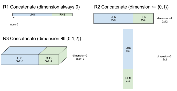
1 boyutlu örnek:
Concat({ {2, 3}, {4, 5}, {6, 7} }, 0)
>>> {2, 3, 4, 5, 6, 7}
2 boyutlu örnek:
let a = {
{1, 2},
{3, 4},
{5, 6},
};
let b = {
{7, 8},
};
Concat({a, b}, 0)
>>> {
{1, 2},
{3, 4},
{5, 6},
{7, 8},
}
Diyagram:
Şart Kipi
Ayrıca bkz.
XlaBuilder::Conditional.
Conditional(pred, true_operand, true_computation, false_operand,
false_computation)
| Bağımsız değişkenler | Tür | Anlambilim |
|---|---|---|
pred |
XlaOp |
PRED türünde skaler |
true_operand |
XlaOp |
\(T_0\)türündeki bağımsız değişken |
true_computation |
XlaComputation |
\(T_0 \to S\)türünde XlaComputation |
false_operand |
XlaOp |
\(T_1\)türündeki bağımsız değişken |
false_computation |
XlaComputation |
\(T_1 \to S\)türünde XlaComputation |
pred true ise true_computation, pred false ise false_computation yürütülür ve sonucu döndürür.
true_computation, \(T_0\) türünde tek bir bağımsız değişken almalıdır ve aynı türde olması gereken true_operand ile çağrılır. false_computation, \(T_1\) türünde tek bir bağımsız değişken almalı ve aynı türde olması gereken false_operand ile çağrılacaktır. Döndürülen true_computation ve false_computation değerinin türü aynı olmalıdır.
pred değerine bağlı olarak true_computation ve false_computation özelliklerinden yalnızca birinin yürütüleceğini unutmayın.
Conditional(branch_index, branch_computations, branch_operands)
| Bağımsız değişkenler | Tür | Anlambilim |
|---|---|---|
branch_index |
XlaOp |
S32 türünde skaler |
branch_computations |
N XlaComputation dizisi |
\(T_0 \to S , T_1 \to S , ..., T_{N-1} \to S\)türündeki XlaComputations |
branch_operands |
N XlaOp dizisi |
\(T_0 , T_1 , ..., T_{N-1}\)türündeki bağımsız değişkenler |
branch_computations[branch_index] öğesini çalıştırır ve sonucu döndürür. branch_index, < 0 veya >= N olan bir S32 ise branch_computations[N-1] varsayılan dal olarak yürütülür.
Her branch_computations[b], \(T_b\) türünde tek bir bağımsız değişken almalıdır ve aynı türde olması gereken branch_operands[b] ile çağrılır. Her branch_computations[b] için döndürülen değerin türü aynı olmalıdır.
branch_index değerine bağlı olarak branch_computations işlemlerinden yalnızca birinin yürütüleceğini unutmayın.
Dönş. (kıvrım)
Ayrıca bkz.
XlaBuilder::Conv.
ConvWithGeneralPadding gibidir ancak dolgu, kısa şekilde SAME veya Valid olarak belirtilir. AYNI dolgu, girişi (lhs) sıfırlarla doldurur. Böylece çıkış, dikkate alınmadığında girişle aynı şekle sahip olur. GEÇERLİ dolgu, dolgu olmadığı anlamına gelir.
ConvWithGeneralPadding (convolution)
Ayrıca bkz.
XlaBuilder::ConvWithGeneralPadding.
Nöral ağlarda kullanılan türde bir konvolüsyon hesaplar. Burada, konvolüsyon, n boyutlu bir taban alanında hareket eden n boyutlu bir pencere olarak düşünülebilir ve pencerenin her olası konumu için bir hesaplama yapılır.
| Bağımsız değişkenler | Tür | Anlambilim |
|---|---|---|
lhs |
XlaOp |
n+2 giriş dizisini sırala |
rhs |
XlaOp |
n+2 çekirdek ağırlığı dizisini sırala |
window_strides |
ArraySlice<int64> |
n-d çekirdek adımları dizisi |
padding |
ArraySlice< pair<int64,int64>> |
(düşük, yüksek) dolgu n-d dizisi |
lhs_dilation |
ArraySlice<int64> |
n-d lhs genişletme faktörü dizisi |
rhs_dilation |
ArraySlice<int64> |
n-d rhs genişleme faktörü dizisi |
feature_group_count |
int64 | özellik gruplarının sayısı |
batch_group_count |
int64 | Grup gruplarının sayısı |
Uzamsal boyutların sayısı n olsun. lhs bağımsız değişkeni, temel alanı açıklayan bir sıralama n+2 dizisidir. Elbette rhs aynı zamanda bir girdi olsa da buna girdi denir. Bir nöral ağda, bunlar giriş aktivasyonlarıdır.
n+2 boyutları şu sırayla bulunur:
batch: Bu boyuttaki her koordinat, konvolüsyonun gerçekleştiği bağımsız bir girişi temsil eder.z/depth/features: Temel alandaki her (y,x) konumu, kendisiyle ilişkili ve bu boyuta giden bir vektöre sahiptir.spatial_dims: Pencerenin hareket ettiği taban alanını tanımlayannboyutsal boyutunu açıklar.
rhs bağımsız değişkeni, kıvrımlı filtreyi/çekirdek/pencereyi açıklayan bir n+2 sıralaması dizisidir. Boyutlar şu sırayla gösterilir:
output-z: Çıkışınzboyutu.input-z: Bu boyutun ilefeature_group_countçarpımının boyutu, lh cinsindenzboyutunun boyutuna eşit olmalıdır.spatial_dims: Taban alanı boyunca hareket eden n-d penceresini tanımlayannboyutsal boyutunu açıklar.
window_strides bağımsız değişkeni, uzamsal boyutlardaki kıvrımlı pencerenin adımını belirtir. Örneğin, ilk uzamsal boyuttaki adım 3 ise pencere yalnızca ilk uzamsal dizinin 3'e bölünebildiği koordinatlara yerleştirilebilir.
padding bağımsız değişkeni, taban alanına uygulanacak sıfır dolgu miktarını belirtir. Dolgu miktarı negatif olabilir. Negatif dolgunun mutlak değeri, konvolüsyon yapılmadan önce belirtilen boyuttan kaldırılacak öğe sayısını gösterir. padding[0], y boyutunun dolgusunu belirtir ve padding[1], x boyutunun dolgusunu belirtir. Her bir çift, ilk öğe olarak düşük dolguya ve ikinci öğe olarak yüksek dolguya sahiptir. Düşük dolgu, alt dizinlere doğru, yüksek dolgu ise yüksek dizinlere doğru uygulanır. Örneğin, padding[1], (2,3) ise ikinci uzamsal boyutta solda 2 sıfır ve sağda 3 sıfırlık bir dolgu olur. Dolgu kullanmak, evrişimi yapmadan önce aynı sıfır değerlerini girişe (lhs) eklemekle eşdeğerdir.
lhs_dilation ve rhs_dilation bağımsız değişkenleri, her bir boyutsal boyutta sırasıyla lhs ve rhs değerlerine uygulanacak genişleme faktörünü belirtir. Üç boyutlu bir boyuttaki genişletme faktörü d ise ilgili boyuttaki girişlerin her birinin arasına dolaylı olarak d-1 delikleri yerleştirilir ve böylece dizinin boyutu artar. Delikler, işlemsiz bir değerle doldurulur. Bu da evrişim için sıfır anlamına gelir.
Rhs'nin genişlemesi, atröz konvolüsyon olarak da adlandırılır. Daha fazla bilgi için tf.nn.atrous_conv2d bölümünü inceleyin. LH'lerin genişlemesi, ters çevrilmiş konvolüsyon olarak da adlandırılır. Ayrıntılı bilgi için tf.nn.conv2d_transpose başlıklı makaleyi inceleyin.
feature_group_count bağımsız değişkeni (varsayılan değer 1), gruplandırılmış dönüşümler için kullanılabilir. feature_group_count, hem giriş hem de çıkış özelliği boyutunun böleni olmalıdır. feature_group_count 1'den büyükse bu, kavramsal olarak giriş ve çıkış özelliği boyutu ile rhs çıkış özelliği boyutunun, her biri ardışık bir özellik alt dizisinden oluşan birçok feature_group_count grubuna eşit bir şekilde bölündüğü anlamına gelir. rhs öğesinin giriş özelliği boyutunun, lhs giriş özelliği boyutunun feature_group_count değerine bölünmesiyle elde edilen değere eşit olması gerekir (bu nedenle zaten bir giriş özellikleri grubu boyutuna sahiptir). i'inci gruplar, birçok ayrı konvolüsyon için feature_group_count'i hesaplamak üzere birlikte kullanılır. Bu evrimlerin sonuçları, çıktı özelliği boyutunda birleştirilir.
Derinlemesine evrim için feature_group_count bağımsız değişkeni giriş özelliği boyutuna ayarlanır ve [filter_height, filter_width, in_channels, channel_multiplier] olan filtre [filter_height, filter_width, 1, in_channels * channel_multiplier] olarak yeniden şekillendirilir. Daha fazla bilgi için tf.nn.depthwise_conv2d sayfasını inceleyin.
batch_group_count (varsayılan değer 1) bağımsız değişkeni, geri yayılma sırasında gruplandırılmış filtreler için kullanılabilir. batch_group_count, lhs (giriş) toplu boyutunun boyutunun bölen olması gerekir. batch_group_count değeri 1'den büyükse çıktı grubu boyutunun input batch
/ batch_group_count boyutunda olması gerekir. batch_group_count, çıkış özelliği boyutunun böleni olmalıdır.
Çıktı şekli aşağıdaki boyutlara sahiptir ve sırayla gösterilmiştir:
batch: Bu boyutunbatch_group_countile çarpımı,batchboyutunun lh cinsinden boyutuna eşit olmalıdır.z: Çekirdektekioutput-zile aynı boyut (rhs).spatial_dims: Kıvrımlı pencerenin her bir geçerli yerleşimi için bir değer.

Yukarıdaki şekilde batch_group_count alanının işleyiş şekli gösterilmektedir. Verimli bir şekilde, her lh grubunu batch_group_count gruplarına ayırıyor ve aynı işlemi çıkış özellikleri için de yapıyoruz. Ardından, bu grupların her biri için ikili konvolüsyonlar gerçekleştirir ve çıktıyı çıkış özelliği boyutu boyunca birleştiririz. Diğer tüm boyutların (özellik ve mekansal) operasyonel anlamları aynı kalır.
Kıvrımlı pencerenin geçerli yerleşimleri, adımlara ve dolgudan sonraki taban alanının boyutuna göre belirlenir.
Bir evrişimin ne işe yaradığını açıklamak için 2 boyutlu evrişimi dikkate alın ve çıktıda bazı sabit batch, z, y, x koordinatları seçin. Daha sonra (y,x), pencerenin bir köşesinin taban alanı içindeki konumudur (ör. mekansal boyutları nasıl yorumladığınıza bağlı olarak sol üst köşe). Artık, taban alanından alınan ve her 2D noktanın bir 1d vektörle ilişkilendirildiği 2D bir penceremiz vardır. Bu durumda 3D kutu elde ederiz. Konvolüsyonel çekirdekte, z çıkış koordinatını düzelttiğimizden, 3D kutumuz da mevcuttur. İki kutu aynı boyutlara sahiptir. Böylece iki kutu arasındaki öğe düzeyindeki çarpımların toplamını alabiliriz (noktalı çarpıma benzer şekilde). Bu, çıkış değeridir.
output-z, ör. 5 değerini ayarlarsanız pencerenin her konumu, çıktının z boyutunda 5 değer oluşturur. Bu değerler, konvolüsyonel çekirdeğin hangi bölümünün kullanıldığına göre değişir. Her output-z koordinatı için kullanılan ayrı bir 3D değer kutusu vardır. Yani bunu, her biri için farklı bir filtre
içeren 5 ayrı konvolüsyon olarak düşünebilirsiniz.
Burada, dolgu ve çizgili bir 2D evrişim için sözde kod verilmiştir:
for (b, oz, oy, ox) {  // output coordinates
  value = 0;
  for (iz, ky, kx) {  // kernel coordinates and input z
    iy = oy*stride_y + ky - pad_low_y;
    ix = ox*stride_x + kx - pad_low_x;
    if ((iy, ix) inside the base area considered without padding) {
      value += input(b, iz, iy, ix) * kernel(oz, iz, ky, kx);
    }
  }
  output(b, oz, oy, ox) = value;
}
ConvertElementType
Ayrıca bkz.
XlaBuilder::ConvertElementType.
C++'taki öğe düzeyinde static_cast işlemine benzer şekilde, bir veri şeklinden hedef şekline öğe düzeyinde bir dönüşüm işlemi gerçekleştirir. Boyutlar eşleşmelidir ve dönüşüm öğe bazlı bir dönüşümdür. Örneğin, s32 öğeleri, s32-f32 dönüşüm rutini aracılığıyla f32 öğelerine dönüşür.
ConvertElementType(operand, new_element_type)
| Bağımsız değişkenler | Tür | Anlambilim |
|---|---|---|
operand |
XlaOp |
soluk D'leri olan T türü dizisi |
new_element_type |
PrimitiveType |
U yazın |
İşlem görenin boyutları ve hedef şekli eşleşmelidir. Kaynak ve hedef öğe türleri "tuple" olmamalıdır.
T=s32-U=f32 gibi bir dönüşüm, yuvarlamadan en yakın eşit değere gibi normalleştirmeden kayma dönüşüm rutini gerçekleştirir.
let a: s32[3] = {0, 1, 2};
let b: f32[3] = convert(a, f32);
then b == f32[3]{0.0, 1.0, 2.0}
CrossReplicaSum
Toplama hesaplamasıyla AllReduce gerçekleştirir.
CustomCall
Ayrıca bkz.
XlaBuilder::CustomCall.
Bir hesaplamada kullanıcı tarafından sağlanan işlevi çağırma.
CustomCall(target_name, args..., shape)
| Bağımsız değişkenler | Tür | Anlambilim |
|---|---|---|
target_name |
string |
İşlevin adı. Bu sembol adını hedefleyen bir çağrı talimatı yayınlanır. |
args |
N XlaOp dizisi |
İşleve aktarılacak rastgele türde N bağımsız değişken. |
shape |
Shape |
İşlevin çıkış şekli |
İşlev imzası, bağımsız değişkenlerin türünden veya bağımsız değişkenlerinden bağımsız olarak aynıdır:
extern "C" void target_name(void* out, void** in);
Örneğin, CustomCall aşağıdaki gibi kullanılıyorsa:
let x = f32[2] {1,2};
let y = f32[2x3] { {10, 20, 30}, {40, 50, 60} };

CustomCall("myfunc", {x, y}, f32[3x3])
Aşağıda, myfunc uygulamasının bir örneği verilmiştir:
extern "C" void myfunc(void* out, void** in) {
  float (&x)[2] = *static_cast<float(*)[2]>(in[0]);
  float (&y)[2][3] = *static_cast<float(*)[2][3]>(in[1]);
  EXPECT_EQ(1, x[0]);
  EXPECT_EQ(2, x[1]);
  EXPECT_EQ(10, y[0][0]);
  EXPECT_EQ(20, y[0][1]);
  EXPECT_EQ(30, y[0][2]);
  EXPECT_EQ(40, y[1][0]);
  EXPECT_EQ(50, y[1][1]);
  EXPECT_EQ(60, y[1][2]);
  float (&z)[3][3] = *static_cast<float(*)[3][3]>(out);
  z[0][0] = x[1] + y[1][0];
  // ...
}
Kullanıcı tarafından sağlanan işlevin yan etkileri bulunmamalı ve çalıştırılması etkili olmalıdır.
Nokta
Ayrıca bkz.
XlaBuilder::Dot.
Dot(lhs, rhs)
| Bağımsız değişkenler | Tür | Anlambilim |
|---|---|---|
lhs |
XlaOp |
T türü dizisi |
rhs |
XlaOp |
T türü dizisi |
Bu işlemin tam anlamı, işlenenlerin sıralamasına bağlıdır:
| Giriş | Çıkış | Anlambilim |
|---|---|---|
vektör [n] dot vektör [n] |
skaler | vektör nokta çarpımı |
matris [m x k] dot vektörü [k] |
vektör [m] | matris vektör çarpım |
matris [m x k] dot matris [k x n] |
matris [m x n] | matris-matris çarpımı |
İşlem, ikinci boyut lhs (veya sıralaması 1 ise birinci boyut) ve ilk boyutu rhs üzerinden ürünlerin toplamını gerçekleştirir. Bunlar "taahhütlü" boyutlardır. lhs ve rhs taahhütlü boyutları aynı boyutta olmalıdır. Pratikte vektörler arasında nokta çarpımları, vektör/matris çarpımları veya matris/matris çarpımları yapmak için kullanılabilir.
DotGeneral
Ayrıca bkz.
XlaBuilder::DotGeneral.
DotGeneral(lhs, rhs, dimension_numbers)
| Bağımsız değişkenler | Tür | Anlambilim |
|---|---|---|
lhs |
XlaOp |
T türü dizisi |
rhs |
XlaOp |
T türü dizisi |
dimension_numbers |
DotDimensionNumbers |
sözleşme ve parti boyutu numaraları |
Dot'a benzer, ancak hem lhs hem de rhs için sözleşme ve toplu boyut numaralarının belirtilmesini sağlar.
| NoktaBoyut Sayıları Alanları | Tür | Anlambilim |
|---|---|---|
lhs_contracting_dimensions
|
tekrar eden int64 | lhs sözleşme boyutu
numarası |
rhs_contracting_dimensions
|
tekrar eden int64 | rhs sözleşme boyutu
numarası |
lhs_batch_dimensions
|
tekrar eden int64 | lhs grup boyut
numarası |
rhs_batch_dimensions
|
tekrar eden int64 | rhs grup boyut
numarası |
DotGeneral, dimension_numbers içinde belirtilen sözleşme boyutları yerine ürünlerin toplamını gerçekleştirir.
lhs ve rhs kaynaklı ilişkilendirilmiş sözleşme boyutu numaralarının aynı olması gerekmez ancak boyut boyutları aynı olmalıdır.
Taahhütlü boyut numaralarıyla örnek:
lhs = { {1.0, 2.0, 3.0},
{4.0, 5.0, 6.0} }

rhs = { {1.0, 1.0, 1.0},
{2.0, 2.0, 2.0} }

DotDimensionNumbers dnums;
dnums.add_lhs_contracting_dimensions(1);
dnums.add_rhs_contracting_dimensions(1);

DotGeneral(lhs, rhs, dnums) -> { {6.0, 12.0},
{15.0, 30.0} }
lhs ve rhs kapsamındaki ilişkilendirilen toplu boyut numaraları aynı boyut boyutlarına sahip olmalıdır.
Grup boyut numaraları (toplu boyutu 2, 2x2 matrisler) içeren örnek:
lhs = { { {1.0, 2.0},
{3.0, 4.0} },
{ {5.0, 6.0},
{7.0, 8.0} } }

rhs = { { {1.0, 0.0},
{0.0, 1.0} },
{ {1.0, 0.0},
{0.0, 1.0} } }

DotDimensionNumbers dnums;
dnums.add_lhs_contracting_dimensions(2);
dnums.add_rhs_contracting_dimensions(1);
dnums.add_lhs_batch_dimensions(0);
dnums.add_rhs_batch_dimensions(0);

DotGeneral(lhs, rhs, dnums) -> { { {1.0, 2.0},
{3.0, 4.0} },
{ {5.0, 6.0},
{7.0, 8.0} } }
| Giriş | Çıkış | Anlambilim |
|---|---|---|
[b0, m, k] dot [b0, k, n] |
[b0, e, n] | toplu matmul |
[b0, b1, m, k] dot [b0, b1, k, n] |
[b0, b1, m, n] | toplu matmul |
Elde edilen boyut numarasının toplu boyutla başlaması, lhs sözleşmesiz/toplu olmayan boyutu ve son olarak da rhs sözleşmesiz/toplu olmayan boyutuyla sonuçlandığı sonucuna varılır.
DynamicSlice
Ayrıca bkz.
XlaBuilder::DynamicSlice.
DynamicSlice, dinamik start_indices konumundaki giriş dizisinden bir alt dizi çıkarır. Her boyuttaki dilimin boyutu size_indices içinde iletilir. Bu özellik, her boyuttaki özel dilim aralıklarının bitiş noktasını belirtir: [başlangıç, başlangıç + boyut). start_indices şekli sıralama ==1 olmalı ve boyut boyutu operand sıralamasına eşit olmalıdır.
DynamicSlice(operand, start_indices, size_indices)
| Bağımsız değişkenler | Tür | Anlambilim |
|---|---|---|
operand |
XlaOp |
T türünde N boyutlu dizi |
start_indices |
N XlaOp dizisi |
Her boyut için dilimin başlangıç dizinlerini içeren N skaler tam sayının listesi. Değer sıfırdan büyük veya sıfıra eşit olmalıdır. |
size_indices |
ArraySlice<int64> |
Her boyut için dilim boyutunu içeren N tam sayıdan oluşan liste. Modül boyut boyutunun sarmalanmasını önlemek için her değer kesinlikle sıfırdan büyük olmalı ve başlangıç + boyutu, boyutun boyutundan küçük veya ona eşit olmalıdır. |
Etkili dilim dizinleri, dilimi gerçekleştirmeden önce [1, N) içindeki her bir dizin i için aşağıdaki dönüşüm uygulanarak hesaplanır:
start_indices[i] = clamp(start_indices[i], 0, operand.dimension_size[i] - size_indices[i])
Bu, çıkarılan dilimin işlenen diziye göre her zaman sınır içinde olmasını sağlar. Dönüşüm uygulanmadan önce dilim sınırların içindeyse dönüşümün herhangi bir etkisi olmaz.
1 boyutlu örnek:
let a = {0.0, 1.0, 2.0, 3.0, 4.0}
let s = {2}

DynamicSlice(a, s, {2}) produces:
{2.0, 3.0}
2 boyutlu örnek:
let b =
{ {0.0,  1.0,  2.0},
{3.0,  4.0,  5.0},
{6.0,  7.0,  8.0},
{9.0, 10.0, 11.0} }
let s = {2, 1}

DynamicSlice(b, s, {2, 2}) produces:
{ { 7.0,  8.0},
{10.0, 11.0} }
DynamicUpdateSlice
Ayrıca bkz.
XlaBuilder::DynamicUpdateSlice.
DynamicUpdateSlice, operand giriş dizisinin değeri olan bir sonuç oluşturur ve start_indices konumunda bir update diliminin üzerine yazılır.
update şekli, güncellenen sonucun alt dizisinin şeklini belirler.
start_indices şekli sıralama == 1 olmalı ve boyut boyutu operand sıralamasına eşit olmalıdır.
DynamicUpdateSlice(operand, update, start_indices)
| Bağımsız değişkenler | Tür | Anlambilim |
|---|---|---|
operand |
XlaOp |
T türünde N boyutlu dizi |
update |
XlaOp |
Dilim güncellemesini içeren T türünde N boyutlu dizi. Sınır dışında güncelleme dizinleri oluşturulmasını önlemek amacıyla, güncelleme şeklinin her boyutu kesinlikle sıfırdan büyük olmalı ve başlangıç + güncelleme, her boyutun işlenen boyutundan küçük veya ona eşit olmalıdır. |
start_indices |
N XlaOp dizisi |
Her boyut için dilimin başlangıç dizinlerini içeren N skaler tam sayının listesi. Değer sıfırdan büyük veya sıfıra eşit olmalıdır. |
Etkili dilim dizinleri, dilimi gerçekleştirmeden önce [1, N) içindeki her bir dizin i için aşağıdaki dönüşüm uygulanarak hesaplanır:
start_indices[i] = clamp(start_indices[i], 0, operand.dimension_size[i] - update.dimension_size[i])
Bu, güncellenen dilimin işlenen diziye göre her zaman sınır içinde olmasını sağlar. Dönüşüm uygulanmadan önce dilim sınırların içindeyse dönüşümün herhangi bir etkisi olmaz.
1 boyutlu örnek:
let a = {0.0, 1.0, 2.0, 3.0, 4.0}
let u = {5.0, 6.0}
let s = {2}

DynamicUpdateSlice(a, u, s) produces:
{0.0, 1.0, 5.0, 6.0, 4.0}
2 boyutlu örnek:
let b =
{ {0.0,  1.0,  2.0},
{3.0,  4.0,  5.0},
{6.0,  7.0,  8.0},
{9.0, 10.0, 11.0} }
let u =
{ {12.0,  13.0},
{14.0,  15.0},
{16.0,  17.0} }

let s = {1, 1}

DynamicUpdateSlice(b, u, s) produces:
{ {0.0,  1.0,  2.0},
{3.0, 12.0, 13.0},
{6.0, 14.0, 15.0},
{9.0, 16.0, 17.0} }
Element bazında ikili aritmetik işlemler
Ayrıca bkz.
XlaBuilder::Add.
Öğe bazında bir dizi ikili aritmetik işlem desteklenir.
Op(lhs, rhs)
Burada Op şunlardan biridir: Add (toplama), Sub (çıkarma), Mul (çarpma), Div (bölme), Rem (kalan), Max (maksimum), Min (minimum), LogicalAnd (mantıksal VE) veya LogicalOr (mantıksal VEYA).
| Bağımsız değişkenler | Tür | Anlambilim |
|---|---|---|
lhs |
XlaOp |
sol taraftaki işlenen: T türü dizisi |
rhs |
XlaOp |
sağ taraftaki işlenen: T türü dizisi |
Bağımsız değişkenlerin şekilleri benzer veya uyumlu olmalıdır. Şekillerin uyumlu olmasının ne anlama geldiği hakkında yayınlama dokümanlarına bakın. Bir işlemin sonucunda, iki giriş dizisinin yayınlanması sonucunda ortaya çıkan bir şekle sahip olur. Bu varyantta, işlenenlerden biri skaler olmadığı sürece farklı sıralamalardaki diziler arasındaki işlemler desteklenmez.
Op Rem olduğunda sonuç işareti bölmeden alınır ve sonucun mutlak değeri her zaman bölenin mutlak değerinden küçük olur.
Tam sayı bölme taşması (imzalı/imzasız bölme/sıfır şeklinde kalan veya -1 ile imzalanmış bölüm/kalan INT_SMIN), uygulama tanımlı bir değer üretir.
Bu işlemler için farklı sıralamaya sahip yayın desteğine sahip alternatif bir varyant vardır:
Op(lhs, rhs, broadcast_dimensions)
Burada Op yukarıdakiyle aynıdır. İşlemin bu varyantı, farklı sıralamalardaki diziler arasındaki aritmetik işlemler (ör. vektöre matris ekleme) için kullanılmalıdır.
Ek broadcast_dimensions işleneni, düşük sıralı işlenenin sıralamasını daha yüksek sıralı işlenenin sıralamasına kadar genişletmek için kullanılan bir tam sayı dilimidir. broadcast_dimensions, alt sıralamalı şeklin boyutlarını üst sıradaki şeklin boyutlarıyla eşler. Genişletilmiş şeklin eşlenmemiş boyutları birinci
boyutlarla doldurulur. Bozuk boyut yayını daha sonra, her iki işlenen boyutun şekillerini eşitlemek için bu bozuk boyutlar boyunca şekiller yayınlar. Anlamlar, yayın sayfasında ayrıntılı olarak açıklanmaktadır.
Öğe bazında karşılaştırma işlemleri
Ayrıca bkz.
XlaBuilder::Eq.
Öğe bazında bir grup standart ikili karşılaştırma işlemi desteklenir. Kayan nokta türlerini karşılaştırırken standart IEEE 754 kayan nokta karşılaştırma semantiklerinin geçerli olduğunu unutmayın.
Op(lhs, rhs)
Op şunlardan biridir: Eq (eşittir), Ne (eşit değildir), Ge
(büyüktür veya eşittir), Gt (büyüktür), Le (küçük veya eşittir), Lt
(küçüktür). Diğer bir operatör grubu olan EqTotalOrder, NeTotalOrder, GeTotalOrder, GtTotalOrder, LeTotalOrder ve LtTotalOrder ise -NaN < -Inf < -Finite < -0 < +0 <N +Fini kullanarak kayan nokta numaralarından daha fazla toplam siparişi destekleme haricinde aynı işlevleri sunmaktadır.
| Bağımsız değişkenler | Tür | Anlambilim |
|---|---|---|
lhs |
XlaOp |
sol taraftaki işlenen: T türü dizisi |
rhs |
XlaOp |
sağ taraftaki işlenen: T türü dizisi |
Bağımsız değişkenlerin şekilleri benzer veya uyumlu olmalıdır. Şekillerin uyumlu olmasının ne anlama geldiği hakkında yayınlama dokümanlarına bakın. Bir işlemin sonucunda, iki giriş dizisinin PRED öğe türüyle yayınlanması sonucunda bir şekle sahip olur. Bu varyantta, işlenenlerden biri skaler olmadığı sürece farklı sıralamalardaki diziler arasındaki işlemler desteklenmez.
Bu işlemler için farklı sıralamaya sahip yayın desteğine sahip alternatif bir varyant vardır:
Op(lhs, rhs, broadcast_dimensions)
Burada Op yukarıdakiyle aynıdır. İşlemin bu varyantı, farklı sıralamalardaki diziler arasındaki karşılaştırma işlemleri (ör. vektöre matris ekleme) için kullanılmalıdır.
Ek broadcast_dimensions işleneni, işlenenleri yayınlamak için kullanılacak boyutları belirten bir tam sayı dilimidir. Anlamlar, yayın sayfasında ayrıntılı olarak açıklanmaktadır.
Öğe bazında tekli fonksiyonlar
XlaBuilder, öğe açısından şu tekli işlevleri destekler:
Abs(operand) Öğe bazında mutlak x -> |x|.
Ceil(operand) Element olarak tavan x -> ⌈x⌉.
Cos(operand) Öğe bazında kosinüs x -> cos(x).
Exp(operand) Öğe olarak doğal üstel x -> e^x.
Floor(operand) Öğe bazında x -> ⌊x⌋.
Imag(operand) Karmaşık (veya gerçek) bir şeklin öğe bazında hayali bir parçası. x -> imag(x). İşlem gören bir kayan nokta türündeyse 0 değerini döndürür.
IsFinite(operand) Her bir operand öğesinin sonlu olup olmadığını, yani pozitif veya negatif sonsuz olup olmadığını ve NaN olup olmadığını test eder. Girişle aynı şekle sahip PRED değerleri dizisi döndürür. Burada her öğe, yalnızca karşılık gelen giriş öğesi sonluysa true olur.
Log(operand) Öğe olarak doğal logaritma x -> ln(x).
LogicalNot(operand) Öğe olarak mantıksal değil x -> !(x).
Logistic(operand) Öğe bazında mantıksal fonksiyon hesaplaması x ->
logistic(x).
PopulationCount(operand) operand öğesinin her bir öğesinde ayarlanan bit sayısını hesaplar.
Neg(operand) Öğe bazında olumsuzlama x -> -x.
Real(operand) Karmaşık (veya gerçek) bir şeklin öğe olarak gerçek kısmı.
x -> real(x). İşlem gören bir kayan nokta türüyse aynı değeri döndürür.
Rsqrt(operand) Karekök işleminin öğe bazında tersi
x -> 1.0 / sqrt(x).
Sign(operand) Öğe bazında işaret işlemi x -> sgn(x) burada:
\[\text{sgn}(x) = \begin{cases} -1 & x < 0\\ -0 & x = -0\\ NaN & x = NaN\\ +0 & x = +0\\ 1 & x > 0 \end{cases}\]
operand öğe türünün karşılaştırma operatörünü kullanarak.
Sqrt(operand) Öğe bazında karekök işlemi x -> sqrt(x).
Cbrt(operand) Öğe bazında kübik kök işlemi x -> cbrt(x).
Tanh(operand) Element olarak hiperbolik tanjant x -> tanh(x).
Round(operand) Öğe bazında yuvarlama, sıfırdan uzaklaşır.
RoundNearestEven(operand) Öğe bazında yuvarlama, en yakın çifte bağlanır.
| Bağımsız değişkenler | Tür | Anlambilim |
|---|---|---|
operand |
XlaOp |
İşlevin işleneni |
İşlev, operand dizisindeki her öğeye uygulanır ve aynı şekle sahip bir dizi elde edilir. operand değerinin skaler olmasına izin verilir (sıralama 0).
FF
XLA FFT işlemi, gerçek ve karmaşık girişler/çıkışlar için ileriye ve ters Fourier Dönüşümlerini uygular. En fazla 3 eksende çok boyutlu FFT'ler desteklenir.
Ayrıca bkz.
XlaBuilder::Fft.
| Bağımsız değişkenler | Tür | Anlambilim |
|---|---|---|
operand |
XlaOp |
Fourier'in dönüştürdüğü dizi. |
fft_type |
FftType |
Aşağıdaki tabloya bakın. |
fft_length |
ArraySlice<int64> |
Dönüştürülen eksenlerin zaman alanı uzunlukları. RFFT(fft_length=[16]), RFFT(fft_length=[17]) ile aynı çıktı şekline sahip olduğundan bu, özellikle IRFFT'nin en iç ekseni doğru boyutlandırması için gereklidir. |
FftType |
Anlambilim |
|---|---|
FFT |
Karmaşıktan karmaşık FFT'ye yönlendirme. Şekil değişmedi. |
IFFT |
Ters karmaşıktan karmaşığa FFT. Şekil değişmedi. |
RFFT |
Gerçekten karmaşıka FFT'ye yönlendirin. fft_length[-1] sıfır olmayan bir değerse en içteki eksenin şekli fft_length[-1] // 2 + 1 olur. Değer, Nyquist frekansından sonra dönüştürülen sinyalin ters eşleştirilmiş kısmı hariç tutulur. |
IRFFT |
Ters gerçeğe doğru karmaşık FFT (yani karmaşıktır, gerçek sonucunu döndürür). fft_length[-1] sıfır olmayan bir değerse en içteki eksenin şekli fft_length[-1] olarak genişletilir. Burada, dönüştürülen sinyalin 1 ile fft_length[-1] // 2 + 1 girişlerinin ters eşleniğinden Nyquist frekansı ötesindeki bölümü çıkarım yapılır. |
Çok boyutlu FFT
1'den fazla fft_length sağlandığında bu, en içteki eksenlerin her birine bir basamak FFT işlemi uygulamaya eşdeğerdir. Gerçek->karmaşık ve karmaşık->gerçek durumlarda, en içteki eksen dönüşümü etkili bir şekilde ilk sırada (RFFT; en sonda IRFFT) gerçekleştirilir. Bu nedenle, en içteki eksenin boyutu değişen taraf olduğunu unutmayın. Diğer eksen dönüşümleri ise
karmaşık hale gelir.
Uygulama ayrıntıları
CPU FFT, Eigen'in TensorFFT'si tarafından desteklenir. GPU FFT, cuFFT kullanır.
Topla
XLA, bir giriş dizisinin birkaç dilimini (her bir dilim potansiyel olarak farklı bir çalışma zamanı ofsetinde) bir araya getirir.
Genel Anlambilim
Ayrıca bkz.
XlaBuilder::Gather.
Daha kolay anlaşılır bir açıklama için aşağıdaki "Resmi Olmayan Açıklama" bölümüne bakın.
gather(operand, start_indices, offset_dims, collapsed_slice_dims, slice_sizes, start_index_map)
| Bağımsız değişkenler | Tür | Anlambilim |
|---|---|---|
operand |
XlaOp |
Topladığımız dizi. |
start_indices |
XlaOp |
Topladığımız dilimlerin başlangıç dizinlerini içeren dizi. |
index_vector_dim |
int64 |
start_indices içinde, başlangıç dizinlerini "içeren" boyut. Ayrıntılı açıklama için aşağıya bakın. |
offset_dims |
ArraySlice<int64> |
Çıktı şeklinde yer alan ve işlenenden ayrılmış bir dizi şeklinde belirli uzaklıktaki boyutlar. |
slice_sizes |
ArraySlice<int64> |
slice_sizes[i], i boyutundaki dilimin sınırlarıdır. |
collapsed_slice_dims |
ArraySlice<int64> |
Her bir dilimdeki daraltılmış boyut kümesi. Bu boyutların boyutu 1 olmalıdır. |
start_index_map |
ArraySlice<int64> |
start_indices içindeki dizinlerin yasal dizinlerle işlenen dizinlerle nasıl eşleneceğini açıklayan bir harita. |
indices_are_sorted |
bool |
Dizinlerin arayana göre sıralanmasının garanti edilip edilmediği. |
unique_indices |
bool |
Arayan kişi dizinlerin benzersiz olacağını garanti edip etmediği. |
Kolaylık sağlamak için offset_dims içinde olmayan çıkış dizisindeki boyutları batch_dims olarak etiketleriz.
Çıktı, batch_dims.size + offset_dims.size sıralaması dizisidir.
operand.rank, offset_dims.size ile collapsed_slice_dims.size toplamına eşit olmalıdır. Ayrıca slice_sizes.size, operand.rank değerine eşit olmalıdır.
index_vector_dim, start_indices.rank'a eşitse dolaylı olarak start_indices öğesinin sonda bir 1 boyutu olduğunu kabul ederiz (ör. start_indices, [6,7] biçiminde ve index_vector_dim 2 ise, dolaylı olarak start_indices şeklini [6,7,1] olarak kabul ederiz).
i boyutu boyunca çıkış dizisinin sınırları şu şekilde hesaplanır:
i,batch_dimsiçinde mevcutsa (yani bazıkiçinbatch_dims[k]değerine eşitse)start_indices.shapeüzerinden karşılık gelen boyut sınırlarını seçeriz veindex_vector_dimatlanır (yanik<index_vector_dimisestart_indices.shape.dims[k] ve aksi haldestart_indices.shape.dims[k+1]).i,offset_dimsiçinde mevcutsa (yani bazıkiçinoffset_dims[k] değerine eşitse)collapsed_slice_dimshesaba katıldıktan sonraslice_sizesüzerinden karşılık gelen sınırı seçeriz (yani,collapsed_slice_dimsdizindeki sınırlar kaldırıldığındaadjusted_slice_sizesslice_sizesolduğuadjusted_slice_sizes[k] değerini seçeriz).
Resmi olarak, belirli bir çıkış dizinine (Out) karşılık gelen In işlenen dizini şu şekilde hesaplanır:
kiçinbatch_dims} içinG= {Out[k] bırakın.S[i] =start_indices[Birleştir(G,i)] olacak şekildeSvektörünü ayırmak içinGkullanın. Burada Birleştirme(A; b),index_vector_dimkonumundaki b'yi A konumuna ekler.Gboş olsa bile bunun iyi bir şekilde tanımlandığını unutmayın:GboşsaS=start_indicesolur.start_index_mapkullanarakSöğesini dağıtarakSinileSöğesini kullanarak bir başlangıç dizini (Sin) oluşturun.operandDaha kesin olarak:k<start_index_map.sizeiseSin[start_index_map[k]] =S[k].Sin[_] =0aksi takdirde.
Dizinleri,
collapsed_slice_dimskümesine göreOutöğesindeki ofset boyutlarında dağıtarakoperandiçinOinşeklinde bir dizin oluşturun. Daha kesin olarak:Oin[remapped_offset_dims(k)] =Outk<offset_dims.sizeise (remapped_offset_dimsaşağıda tanımlanmıştır).koffset_dimsOin[_] =0aksi takdirde.
In,Oin+Sinşeklindedir. Burada +, öğe düzeyinde toplamadır.
remapped_offset_dims, alan adı [0,
offset_dims.size) ve aralığı [0, operand.rank) \ collapsed_slice_dims ile monotonik bir fonksiyondur. Örneğin, offset_dims.size 4, operand.rank 6 ve
collapsed_slice_dims {0, 2}, ardından remapped_offset_dims {0→1,
1→3, 2→4, 3→5}.
indices_are_sorted doğru değerine ayarlanırsa XLA, start_indices öğesinin kullanıcı tarafından (artan start_index_map düzende) sıralandığını varsayabilir. Eşleşmezlerse anlamlar
uygulama olarak tanımlanır.
unique_indices, doğru değerine ayarlanırsa XLA, dağınık haldeki tüm öğelerin benzersiz olduğunu varsayabilir. Yani XLA, atomik olmayan işlemleri kullanabilir. unique_indices true (doğru) değerine ayarlanırsa ve dağılan dizinler benzersiz değilse semantik uygulama tanımlanır.
Gayri resmî Açıklama ve Örnekler
Gayriresmi olarak çıkış dizisindeki her dizin Out, işlenen dizideki bir E öğesine karşılık gelir. Aşağıdaki şekilde hesaplanır:
start_indicesbaşlangıç dizinini aramak içinOutöğesindeki grup boyutlarını kullanırız.Başlangıç dizinini (boyutu operand.rank değerinden küçük olabilir) "tam" başlangıç diziniyle
operandarasında eşlemek içinstart_index_mapkullanırız.Tam başlangıç dizinini kullanarak,
slice_sizesboyutunda bir dilimi dinamik olarak böleriz.collapsed_slice_dimsboyutları daraltılarak dilimi yeniden şekillendiririz. Tüm daraltılmış dilim boyutlarının sınırı 1 olması gerektiğinden, bu yeniden şekil her zaman yasaldır.Çıkış dizinine
Outkarşılık gelen giriş öğesini (E) elde etmek üzere bu dilimde dizine eklemek içinOutofset boyutlarını kullanırız.
index_vector_dim, sonraki tüm örneklerde start_indices.rank - 1 olarak ayarlanmıştır. index_vector_dim için daha ilginç değerler işlemi temelde değiştirmez ancak görsel temsili daha zahmetli hale getirir.
Yukarıdakilerin tümünün nasıl birbirine uyduğuna dair bir sezgi elde etmek için [16,11] dizisinden 5 şekil [8,6] şekli toplayan bir örneğe bakalım. Bir dilimin [16,11] dizisindeki konumu, S64[2] şeklinin dizin vektörü olarak temsil edilebilir. Böylece 5 konum kümesi S64[5,2] dizisi olarak temsil edilebilir.
Ardından toplama işleminin davranışı, [G,O0,O1] değerini, çıkış biçimindeki bir dizini alan ve bunu aşağıdaki şekilde giriş dizisindeki bir öğeyle eşleyen bir dizin dönüşümü olarak gösterilebilir:

İlk olarak, G kullanarak toplama dizinleri dizisinden bir (X,Y) vektör seçeriz.
Daha sonra [G,O0,O1] dizinindeki çıkış dizisindeki öğe, [X+O0,Y+O1] dizinindeki giriş dizisindeki öğe olur.
slice_sizes, O0 ve O1 aralığını belirleyen [8,6] değeridir. Bu da dilimin sınırlarını belirler.
Bu toplama işlemi, toplu boyut olarak G ile toplu bir dinamik dilim görevi görür.
Toplama dizinleri çok boyutlu olabilir. Örneğin, yukarıdaki örneğin [4,5,2] şeklinde bir "toplayıcı dizin" dizisi kullanan daha genel bir sürümü, dizinleri şuna benzer şekilde çevirir:

Bu da toplu boyut olarak G0 ve G1 şeklinde bir toplu dinamik dilim olarak işlev görür. Dilim boyutu hâlâ [8,6].
XLA'da toplama işlemi, yukarıda ana hatlarıyla açıklanan gayri resmî anlamları aşağıdaki şekillerde genelleştirir:
Çıktı şeklindeki hangi boyutların uzaklık boyutları (son örnekte
O0,O1içeren boyutlar) olacağını yapılandırabiliriz. Çıkış grubu boyutları (son örnekteG0,G1içeren boyutlar), ofset boyutları olmayan çıktı boyutları olarak tanımlanmıştır.Çıkış biçiminde açıkça bulunan çıkış ofseti boyutlarının sayısı, giriş sıralamasından daha küçük olabilir. Açıkça
collapsed_slice_dimsolarak listelenen bu "eksik" boyutların1dilim boyutuna sahip olması gerekir. Bunların dili1olduğundan, onlar için geçerli tek dizin0olur ve bunların ortadan kaldırılması belirsizliğe yol açmaz.Son örnekte, "Aggregate Indices" dizisinden ((
X,Y) elde edilen dilim), giriş dizisi sıralamasından daha az öğeye sahip olabilir ve açık bir eşleme, dizinin girişle aynı sıralamaya sahip olacak şekilde nasıl genişletileceğini belirler.
Son bir örnek olarak, tf.gather_nd öğesini uygulamak için (2) ve (3) değerlerini kullanırız:

G0 ve G1, başlangıç dizininin yalnızca bir öğesi (X) içermesi dışında, toplama dizinleri dizisinden bir başlangıç dizinini her zamanki gibi ayırmak için kullanılır. Benzer şekilde, O0 değerine sahip yalnızca bir çıkış ofset dizini var. <br-> class="br-y-e-postal{0}<br><-ph-2-2-2">üz düğmesini <br class="br-ph-2-1"><br class="br-ph-2-1"><br class="br-ph-2-1"><br class="br-ph-2-1"><br class="br-2-1">üzerinde asılı<br class="br-ph-2-1"><br class="br-ph-2-1"><br class="br-ph-2-1"><br class="br-ph-2-1"><br class="br-ph-2-1">üzerindestart_index_mapremapped_offset_dimsXX000000000OOOOGGGG11GatherIndicestf.gather_nd
Bu destek kaydı için slice_sizes: [1,11]. Bu, sezgisel olarak toplama dizinleri dizisindeki her dizinin (X) bütün bir satırı seçtiği ve sonucun tüm bu satırların birleştirilmesi anlamına gelir.
GetDimensionSize
Ayrıca bkz.
XlaBuilder::GetDimensionSize.
İşlem gören için belirli bir boyutun boyutunu döndürür. İşlem gören dizi şeklinde olmalıdır.
GetDimensionSize(operand, dimension)
| Bağımsız değişkenler | Tür | Anlambilim |
|---|---|---|
operand |
XlaOp |
n boyutlu giriş dizisi |
dimension |
int64 |
[0, n) aralığında olan ve boyutu belirten bir değer |
SetDimensionSize
Ayrıca bkz.
XlaBuilder::SetDimensionSize.
XlaOp'un verilen boyutunun dinamik boyutunu ayarlar. İşlem gören dizi şeklinde olmalıdır.
SetDimensionSize(operand, size, dimension)
| Bağımsız değişkenler | Tür | Anlambilim |
|---|---|---|
operand |
XlaOp |
n boyutlu giriş dizisi. |
size |
XlaOp |
int32 değeri, çalışma zamanı dinamik boyutunu temsil eder. |
dimension |
int64 |
[0, n) aralığında boyutu belirten bir değer. |
Sonuç olarak, derleyici tarafından izlenen dinamik boyutla işlenen işleneni geçirin.
Doldurulmuş değerler, aşağı akış azaltma işlemleri tarafından yoksayılır.
let v: f32[10] = f32[10]{1, 2, 3, 4, 5, 6, 7, 8, 9, 10};
let five: s32 = 5;
let six: s32 = 6;

// Setting dynamic dimension size doesn't change the upper bound of the static
// shape.
let padded_v_five: f32[10] = set_dimension_size(v, five, /*dimension=*/0);
let padded_v_six: f32[10] = set_dimension_size(v, six, /*dimension=*/0);

// sum == 1 + 2 + 3 + 4 + 5
let sum:f32[] = reduce_sum(padded_v_five);
// product == 1 * 2 * 3 * 4 * 5
let product:f32[] = reduce_product(padded_v_five);

// Changing padding size will yield different result.
// sum == 1 + 2 + 3 + 4 + 5 + 6
let sum:f32[] = reduce_sum(padded_v_six);
GetTupleElement
Ayrıca bkz.
XlaBuilder::GetTupleElement.
Derleme zamanı sabit değerine sahip bir unsura dizine ekler.
Şekil çıkarımının sonuç değerinin türünü belirleyebilmesi için değer bir derleme zaman sabiti olmalıdır.
Bu, C++'taki std::get<int N>(t) yönergesine benzer. Kavramsal olarak:
let v: f32[10] = f32[10]{0, 1, 2, 3, 4, 5, 6, 7, 8, 9};
let s: s32 = 5;
let t: (f32[10], s32) = tuple(v, s);
let element_1: s32 = gettupleelement(t, 1);  // Inferred shape matches s32.
Ayrıca bkz. tf.tuple.
Feed içi
Ayrıca bkz.
XlaBuilder::Infeed.
Infeed(shape)
| Argüman | Tür | Anlambilim |
|---|---|---|
shape |
Shape |
Feed içi arayüzünden okunan verilerin şekli. Şeklin düzen alanı, cihaza gönderilen verilerin düzeniyle eşleşecek şekilde ayarlanmalıdır. Aksi takdirde davranışı tanımlanmamış olur. |
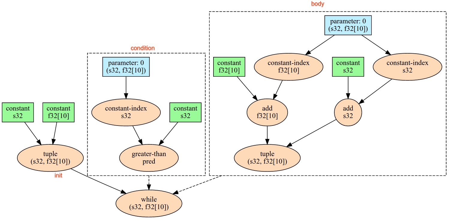
Cihazın dolaylı feed içi akış arayüzünden tek bir veri öğesini okur, verileri belirtilen şekil ve düzeni olarak yorumlar ve verilerin XlaOp kadarını döndürür. Bir hesaplamada birden fazla Feed İçi işleme izin verilir ancak Feed içi işlemler arasında toplam bir sıra olmalıdır. Örneğin, aşağıdaki kodda yer alan iki Feed İçi Reklamın toplam sırası vardır. Bunun nedeni, süre döngüleri arasında bağımlılık olmasıdır.
result1 = while (condition, init = init_value) {
  Infeed(shape)
}

result2 = while (condition, init = result1) {
  Infeed(shape)
}
İç içe yerleştirilmiş tuple şekilleri desteklenmiyor. Boş bir unsur şekli söz konusu olduğunda feed içi işlemi, işlemsiz bir işlemdir ve cihazın feed'inden veri okunmadan devam eder.
Iota
Ayrıca bkz.
XlaBuilder::Iota.
Iota(shape, iota_dimension)
Cihazda potansiyel olarak büyük bir ana makine aktarımı yerine sabit bir değişmez değer oluşturur. Şekli belirtilmiş bir dizi oluşturur ve sıfırdan başlayan ve belirtilen boyut boyunca bir artan değerleri korur. Kayan nokta türlerinde oluşturulan dizi ConvertElementType(Iota(...)) işlevine eş değerdir. Burada Iota integral türünde, dönüşüm ise kayan nokta türüne sahiptir.
| Bağımsız değişkenler | Tür | Anlambilim |
|---|---|---|
shape |
Shape |
Iota() tarafından oluşturulan dizinin şekli |
iota_dimension |
int64 |
Birlikte artırılacak boyut. |
Örneğin, Iota(s32[4, 8], 0) şu değeri döndürür:
  [[0, 0, 0, 0, 0, 0, 0, 0 ],
   [1, 1, 1, 1, 1, 1, 1, 1 ],
   [2, 2, 2, 2, 2, 2, 2, 2 ],
   [3, 3, 3, 3, 3, 3, 3, 3 ]]
Iota(s32[4, 8], 1) karşılığında iade
  [[0, 1, 2, 3, 4, 5, 6, 7 ],
   [0, 1, 2, 3, 4, 5, 6, 7 ],
   [0, 1, 2, 3, 4, 5, 6, 7 ],
   [0, 1, 2, 3, 4, 5, 6, 7 ]]
Harita
Ayrıca bkz.
XlaBuilder::Map.
Map(operands..., computation)
| Bağımsız değişkenler | Tür | Anlambilim |
|---|---|---|
operands |
N XlaOp dizisi |
T0..T{N-1} türünde N dizi |
computation |
XlaComputation |
İsteğe bağlı türde T ve M türünde N parametrelerle T_0, T_1, .., T_{N + M -1} -> S türü hesaplaması |
dimensions |
int64 dizisi |
harita boyutları dizisi |
Verilen operands dizilerine skaler bir işlev uygulayarak her öğenin, giriş dizilerindeki karşılık gelen öğelere uygulanan eşlenmiş işlevin sonucu olduğu aynı boyutlardan bir dizi oluşturur.
Eşlenen işlev, T skalar türde N giriş ve S türünde tek bir çıkışa sahip olması kısıtlamasıyla rastgele bir hesaplamadır. Çıkış, T öğe türünün S ile değiştirilmesi dışında işlenenlerle aynı boyutlara sahiptir.
Örneğin: Map(op1, op2, op3, computation, par1), çıkış dizisini oluşturmak için giriş dizilerindeki her bir (çok boyutlu) dizinde elem_out <-
computation(elem1, elem2, elem3, par1) eşlemesi yapar.
OptimizationBarrier
Herhangi bir optimizasyon geçişinin, hesaplamaları bariyer boyunca taşımasını engeller.
Tüm girişlerin, bariyer çıkışlarına bağlı olan operatörlerden önce değerlendirilmesini sağlar.
Ped
Ayrıca bkz.
XlaBuilder::Pad.
Pad(operand, padding_value, padding_config)
| Bağımsız değişkenler | Tür | Anlambilim |
|---|---|---|
operand |
XlaOp |
T türü dizisi |
padding_value |
XlaOp |
eklenen dolguyu doldurmak için T türünde skaler |
padding_config |
PaddingConfig |
her iki kenardaki (düşük, yüksek) ve her boyutun öğeleri arasındaki dolgu miktarı |
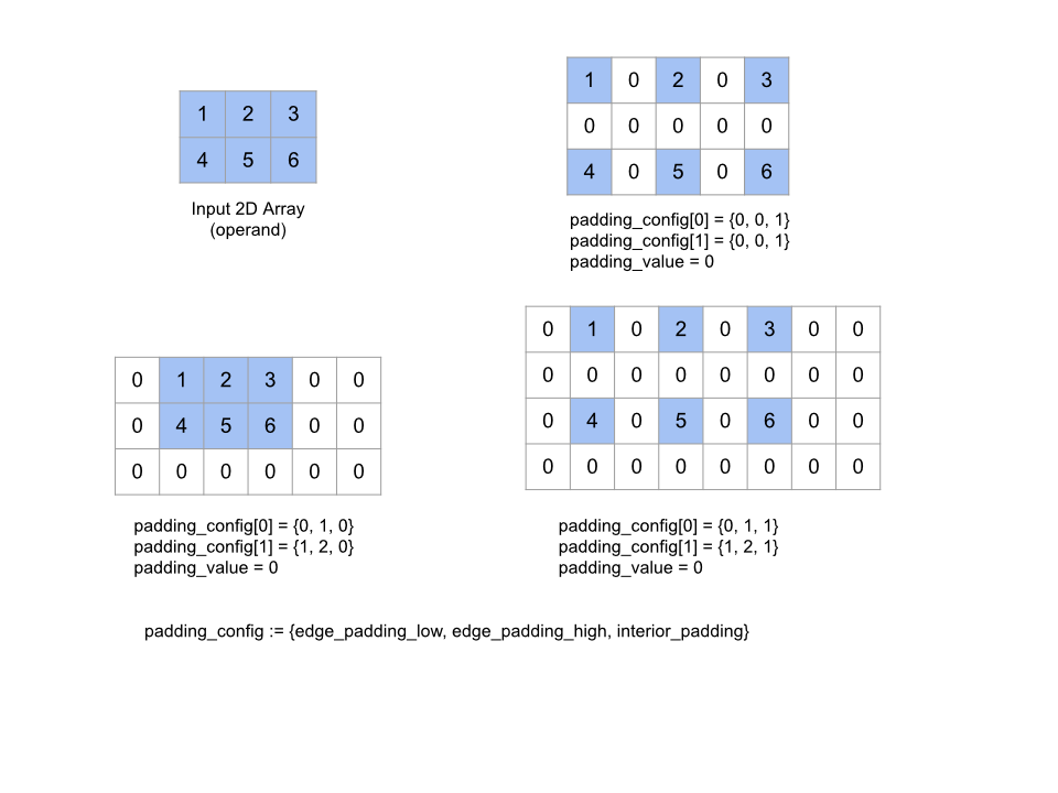
Verilen operand dizisini, dizinin etrafına ve verilen padding_value değerine sahip dizi öğeleri arasına dolgu yaparak genişletir. padding_config, her bir boyut için kenar dolgusu ve iç dolgu miktarını belirtir.
PaddingConfig, her boyut için üç alan içeren yinelenen bir PaddingConfigDimension alanıdır: edge_padding_low, edge_padding_high ve interior_padding.
edge_padding_low ve edge_padding_high, her bir boyutun sırasıyla alt uç (dizin 0'ın yanında) ve üst uç noktasına (en yüksek dizinin yanında) eklenen dolgu miktarını belirtir. Kenar dolgusu miktarı negatif olabilir. Negatif dolgunun mutlak değeri, belirtilen boyuttan kaldırılacak öğe sayısını gösterir.
interior_padding, her bir boyuttaki herhangi iki öğe arasına eklenen dolgu miktarını belirtir. Negatif olamaz. İç dolgu, mantıksal olarak kenar dolgusundan önce gerçekleşir. Bu nedenle, negatif kenar dolgusu durumunda öğeler iç dolgulu işlenenden kaldırılır.
Kenar dolgu çiftlerinin tümü (0, 0) ve iç dolgu değerlerinin tümü 0 ise bu işlem işlemsizdir. Aşağıdaki şekilde, iki boyutlu bir dizi için farklı edge_padding ve interior_padding değerleriyle ilgili örnekler gösterilmektedir.
Alınan
Ayrıca bkz.
XlaBuilder::Recv.
Recv(shape, channel_handle)
| Bağımsız değişkenler | Tür | Anlambilim |
|---|---|---|
shape |
Shape |
istediğiniz verinin şekline |
channel_handle |
ChannelHandle |
her gönder/al çifti için benzersiz tanımlayıcı |
Belirli bir şekle ait verileri, aynı kanal herkese açık kullanıcı adını paylaşan başka bir hesaplamadaki Send talimatından alır. Alınan veriler için bir XlaOp döndürür.
Recv işleminin istemci API'si, eşzamanlı iletişimi temsil eder.
Ancak talimat, eşzamansız veri aktarımlarını etkinleştirmek için dahili olarak 2 HLO talimatlarına (Recv ve RecvDone) ayrılmıştır. Ayrıca bkz.
HloInstruction::CreateRecv ve HloInstruction::CreateRecvDone.
Recv(const Shape& shape, int64 channel_id)
Bir Send talimatından veri almak için gereken kaynakları aynı channel_id ile ayırır. Ayrılan kaynaklar için bir bağlam döndürür. Bu bağlam, veri aktarımının tamamlanmasını beklemek üzere aşağıdaki RecvDone talimatı tarafından kullanılır. Bağlam, {alıcı arabelleği (şekil), istek tanımlayıcısı (U32)} unsurudur ve yalnızca RecvDone talimatı tarafından kullanılabilir.
RecvDone(HloInstruction context)
Recv talimatıyla oluşturulan bir bağlamda, veri aktarımının tamamlanmasını bekler ve alınan verileri döndürür.
Azaltma
Ayrıca bkz.
XlaBuilder::Reduce.
Paralel olarak bir veya daha fazla diziye indirgeme işlevi uygular.
Reduce(operands..., init_values..., computation, dimensions)
| Bağımsız değişkenler | Tür | Anlambilim |
|---|---|---|
operands |
XlaOp. N dizisi |
T_0, ..., T_{N-1} türünde N dizi. |
init_values |
XlaOp. N dizisi |
T_0, ..., T_{N-1} türlerinde N skaler. |
computation |
XlaComputation |
T_0, ..., T_{N-1}, T_0, ..., T_{N-1} -> Collate(T_0, ..., T_{N-1}) türünde hesaplama. |
dimensions |
int64 dizisi |
azaltılacak sırasız boyut dizisi. |
Burada:
- N, 1'den büyük veya 1'e eşit olmalıdır.
- Hesaplamanın "kabaca" ilişkili olması gerekir (aşağıya bakın).
- Tüm giriş dizileri aynı boyutlara sahip olmalıdır.
- Tüm başlangıç değerleri,
computationaltında bir kimlik oluşturmalıdır. N = 1iseCollate(T),Tolur.N > 1iseCollate(T_0, ..., T_{N-1}),TtüründekiNöğelerinin bir unsurudur.
Bu işlem, her bir giriş dizisinin bir veya daha fazla boyutunu skaler boyutlara indirir.
Döndürülen her bir dizinin sıralaması rank(operand) - len(dimensions) şeklindedir. İşlemin çıktısı Collate(Q_0, ..., Q_N) olur. Burada Q_i, boyutları aşağıda açıklanan T_i türünde bir dizidir.
Farklı arka uçların azaltma hesaplamasını yeniden ilişkilendirmesine izin verilir. Toplama gibi bazı azaltma işlevleri, kayan sayılar ile ilişkili olmadığından bu durum sayısal farklılıklara yol açabilir. Bununla birlikte, veri aralığı sınırlıysa kayan nokta ekleme işlemi, çoğu pratik kullanım için ilişki oluşturmaya yetecek kadar yakındır.
Örnekler
Tek bir 1D dizisindeki bir boyutu [10, 11,
12, 13] değerleriyle küçültürken f azaltma işleviyle (bu computation) bu değer şu şekilde hesaplanabilir:
f(10, f(11, f(12, f(init_value, 13)))
ancak daha birçok olasılık da vardır, örneğin,
f(init_value, f(f(10, f(init_value, 11)), f(f(init_value, 12), f(init_value, 13))))
Aşağıda, başlangıç değeri 0 olan indirgenme hesaplaması olarak toplama kullanılarak, azaltmanın nasıl uygulanabileceğine dair kaba bir sözde kod örneği verilmiştir.
result_shape <- remove all dims in dimensions from operand_shape

# Iterate over all elements in result_shape. The number of r's here is equal
# to the rank of the result
for r0 in range(result_shape[0]), r1 in range(result_shape[1]), ...:
  # Initialize this result element
  result[r0, r1...] <- 0

  # Iterate over all the reduction dimensions
  for d0 in range(dimensions[0]), d1 in range(dimensions[1]), ...:
    # Increment the result element with the value of the operand's element.
    # The index of the operand's element is constructed from all ri's and di's
    # in the right order (by construction ri's and di's together index over the
    # whole operand shape).
    result[r0, r1...] += operand[ri... di]
Aşağıda, bir 2D dizinin (matris) indirgenmesine bir örnek verilmiştir. Şeklin sıralaması 2, boyutu 2 için 0, boyutu 3 ve boyutu 3'e sahiptir:
"Ekle" işleviyle 0 veya 1 boyutlarını küçültmenin sonuçları:
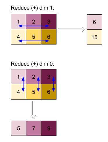
Her iki kısaltma sonucunun da 1D dizileri olduğunu unutmayın. Şemada görsel kolaylık sağlamak için biri sütun, diğeri satır olarak gösterilmektedir.
Daha karmaşık bir örnek için burada bir 3D dizi verilmiştir. Sıralaması 3, boyut 4 için 0 boyut, 2 boyut 1 ve 3 boyut 2 şeklindedir. Basitlik sağlaması açısından, 1 ile 6 arasındaki değerler 0 boyutunda çoğaltılır.
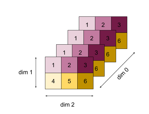
2D örneğine benzer şekilde, yalnızca bir boyutu azaltabiliriz. Örneğin, boyutu 0'ı azaltırsak, boyut 0'daki tüm değerlerin skaler olacak şekilde katlandığı bir sıra-2 dizisi elde ederiz:
|  4   8  12 |
| 16  20  24 |
Boyut 2'yi azaltırsak boyut 2'deki tüm değerlerin skaler olacak şekilde katlandığı bir sıralama 2 dizisi de elde ederiz:
| 6  15 |
| 6  15 |
| 6  15 |
| 6  15 |
Girişteki kalan boyutlar arasındaki göreli sıralamanın çıkışta korunduğunu ancak (sıralama değiştiğinden) bazı boyutlara yeni sayılar atanabileceğini unutmayın.
Ayrıca, birden fazla boyutu küçültebiliriz. Boyut 0 ve 1 azaltıldığında, 1D dizisi [20, 28, 36] oluşturulur.
3D dizisinin tüm boyutlarına göre küçültülmesi skaler 84 sonucunu verir.
Değişken Azaltma
N > 1 olduğunda, azaltma işlevi uygulaması, tüm girişlere aynı anda uygulandığından biraz daha karmaşık hale gelir. İşlem görenler, işleme aşağıdaki sırayla sağlanır:
- İlk işlenen için azaltılmış değer çalıştırılıyor
- ...
- N'inci işlenen için indirimli değer çalıştırılıyor
- İlk işlenen için giriş değeri
- ...
- N'inci işlenen için giriş değeri
Örneğin, 1-D bir dizinin maksimum ve argmax değerini paralel olarak hesaplamak için kullanılabilecek aşağıdaki indirgeme işlevini ele alalım:
f: (Float, Int, Float, Int) -> Float, Int
f(max, argmax, value, index):
  if value >= max:
    return (value, index)
  else:
    return (max, argmax)
1-D Giriş dizileri V = Float[N], K = Int[N] ve başlatma değerleri için
I_V = Float, I_K = Int tek giriş boyutunda azaltmanın f_(N-1) sonucu, şu yinelemeli uygulamaya eşdeğerdir:
f_0 = f(I_V, I_K, V_0, K_0)
f_1 = f(f_0.first, f_0.second, V_1, K_1)
...
f_(N-1) = f(f_(N-2).first, f_(N-2).second, V_(N-1), K_(N-1))
Bu indirgemenin bir değer dizisine ve sıralı dizinler dizisine (ör. iota) uygulanması, diziler üzerinde birlikte iterasyon yapar ve maksimum değer ile eşleşen dizini içeren bir tuple döndürür.
ReducePrecision
Ayrıca bkz.
XlaBuilder::ReducePrecision.
Kayan nokta değerlerini daha düşük duyarlıklı bir biçime (IEEE-FP16 gibi) dönüştürme etkisini modelleyerek orijinal biçime geri döndürür. Daha düşük duyarlıklı biçimde üs ve mantissa bit sayısı isteğe bağlı olarak belirtilebilir ancak tüm donanım uygulamalarında tüm bit boyutları desteklenmeyebilir.
ReducePrecision(operand, mantissa_bits, exponent_bits)
| Bağımsız değişkenler | Tür | Anlambilim |
|---|---|---|
operand |
XlaOp |
T kayan nokta türü dizisi. |
exponent_bits |
int32 |
düşük hassasiyetli biçimde üs bit sayısı |
mantissa_bits |
int32 |
düşük duyarlıklı biçimde mantissa bitlerinin sayısı |
Sonuç, T türünde bir dizidir. Giriş değerleri, verilen mantissa bit sayısı ile temsil edilebilen en yakın değere yuvarlanır ("çift" semantik kullanılarak) ve üs bit sayısı ile belirtilen aralığı aşan değerler pozitif veya negatif sonsuza sabitlenir. NaN değerleri korunur, ancak bu değerler standart NaN değerlerine dönüştürülebilir.
Düşük duyarlıklı biçimde en az bir üs biti bulunmalıdır (sıfır değerinin sonsuzdan ayırt edilebilmesi için her ikisinin de değeri sıfır mantis olmalıdır) ve negatif olmayan bir sayı olmalıdır. Üs veya mantissa bit sayısı, T türünün karşılık gelen değerini aşabilir. Bu durumda dönüşümün karşılık gelen bölümü basitçe işlemsiz durumdadır.
ReduceScatter
Ayrıca bkz.
XlaBuilder::ReduceScatter.
ReduceScatter, etkili bir şekilde bir AllReduce işlemini yapan ve ardından sonucu scatter_dimension boyunca shard_count bloklarına ayırarak dağıtan kolektif bir işlemdir. Ayrıca replika grubundaki i replikası ith parçasını alır.
ReduceScatter(operand, computation, scatter_dim, shard_count,
replica_group_ids, channel_id)
| Bağımsız değişkenler | Tür | Anlambilim |
|---|---|---|
operand |
XlaOp |
Replikalar genelinde azaltılacak dizi veya boş olmayan dizi kümesi. |
computation |
XlaComputation |
Azaltma hesaplaması |
scatter_dimension |
int64 |
Dağılım yapılacak boyut. |
shard_count |
int64 |
Bölünecek blok sayısı scatter_dimension |
replica_groups |
int64 vektörlerinin vektörü |
İndirimlerin yapıldığı gruplar |
channel_id |
isteğe bağlı int64 |
Modüller arası iletişim için isteğe bağlı kanal kimliği |
operandbir dizi unsur olduğunda dağılmayı azaltma işlemi, devirin her bir öğesi üzerinde gerçekleştirilir.replica_groups, azaltmanın gerçekleştirildiği replika gruplarının listesidir (geçerli replikanın replika kimliğiReplicaIdkullanılarak alınabilir). Her gruptaki replikaların sırası, tamamen küçültme sonucunun hangi sırayla dağıtılacağını belirler.replica_groupsya boş olmalı (bu durumda tüm replikalar tek bir gruba ait olmalıdır) ya da replika sayısıyla aynı sayıda öğe içermelidir. Birden fazla replika grubu olduğunda, bunların tümü aynı boyutta olmalıdır. Örneğinreplica_groups = {0, 2}, {1, 3},0ile2replikaları ile1ile3arasında azaltma gerçekleştirir ve daha sonra sonucu dağıtır.shard_count, her bir replika grubunun boyutudur.replica_groupsdeğerinin boş olduğu durumlarda buna ihtiyacımız vardır.replica_groupsboş değilseshard_count, her bir replika grubunun boyutuna eşit olmalıdır.channel_id, modüller arası iletişim için kullanılır: Yalnızca aynıchannel_iddeğerine sahipreduce-scatterişlemleri birbiriyle iletişim kurabilir.
Çıkış şekli, shard_count kat küçültülmüş scatter_dimension ile giriş şeklidir. Örneğin, iki replika varsa ve işlenen iki replikada sırasıyla [1.0, 2.25] ve [3.0, 5.25] değerine sahipse bu işlemde scatter_dim 0 olan çıkış değeri, ilk replika için [4.0], ikinci replika için [7.5] olur.
ReduceWindow
Ayrıca bkz.
XlaBuilder::ReduceWindow.
N adet çok boyutlu dizi dizisinin her bir penceresindeki tüm öğelere bir indirgeme işlevi uygulayarak çıktı olarak N çok boyutlu diziden oluşan tek bir veya bir çift boyutlu dizi üretir. Her çıktı dizisi, pencerenin geçerli konumlarının sayısıyla aynı sayıda öğeye sahiptir. Bir havuz katmanı, ReduceWindow olarak ifade edilebilir. Reduce öğesinde olduğu gibi, uygulanan computation öğesi de sol taraftaki init_values öğesinden her zaman geçer.
ReduceWindow(operands..., init_values..., computation, window_dimensions,
window_strides, padding)
| Bağımsız değişkenler | Tür | Anlambilim |
|---|---|---|
operands |
N XlaOps |
Her biri pencerenin yerleştirildiği temel alanı temsil eden T_0,..., T_{N-1} türünde N çok boyutlu diziden oluşan bir dizi. |
init_values |
N XlaOps |
İndirgemenin N başlangıç değerleri (N işlenenin her biri için bir adet). Ayrıntılar için Azaltma bölümüne bakın. |
computation |
XlaComputation |
Tüm giriş işlenenlerinin her bir penceresindeki öğelere uygulanacak T_0, ..., T_{N-1}, T_0, ..., T_{N-1} -> Collate(T_0, ..., T_{N-1}) türünde azaltma işlevi. |
window_dimensions |
ArraySlice<int64> |
pencere boyutu değerleri için tam sayı dizisi |
window_strides |
ArraySlice<int64> |
pencere adımı değerleri için tam sayı dizisi |
base_dilations |
ArraySlice<int64> |
baz genişleme değerleri için tam sayı dizisi |
window_dilations |
ArraySlice<int64> |
pencere genişletme değerleri için tam sayı dizisi |
padding |
Padding |
pencere için dolgu türü (Dolgu::kAynı, adımın 1 olduğunda girişle aynı çıkış şekline sahip olacak şekilde tamponlar veya dolgu kullanmadığı ve artık sığmadığında pencereyi "durduran" Padding::kValid) |
Burada:
- N, 1'den büyük veya 1'e eşit olmalıdır.
- Tüm giriş dizileri aynı boyutlara sahip olmalıdır.
N = 1iseCollate(T),Tolur.N > 1iseCollate(T_0, ..., T_{N-1}),(T0,...T{N-1})türündekiNöğelerinin bir unsurudur.
Aşağıdaki kod ve şekilde, ReduceWindow kullanımına ilişkin bir örnek gösterilmektedir. Giriş, [4x6] boyutunda bir matristir ve hem window_dimensions hem de window_stride_dimensions [2x3] değerine sahiptir.
// Create a computation for the reduction (maximum).
XlaComputation max;
{
  XlaBuilder builder(client_, "max");
  auto y = builder.Parameter(0, ShapeUtil::MakeShape(F32, {}), "y");
  auto x = builder.Parameter(1, ShapeUtil::MakeShape(F32, {}), "x");
  builder.Max(y, x);
  max = builder.Build().value();
}

// Create a ReduceWindow computation with the max reduction computation.
XlaBuilder builder(client_, "reduce_window_2x3");
auto shape = ShapeUtil::MakeShape(F32, {4, 6});
auto input = builder.Parameter(0, shape, "input");
builder.ReduceWindow(
    input,
    /*init_val=*/builder.ConstantLiteral(LiteralUtil::MinValue(F32)),
    *max,
    /*window_dimensions=*/{2, 3},
    /*window_stride_dimensions=*/{2, 3},
    Padding::kValid);
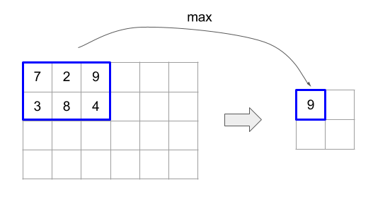
Bir boyuttaki 1'in adımları, boyuttaki bir pencerenin konumunun, bitişik pencereden 1 öğe uzakta olduğunu belirtir. Birbiriyle örtüşen pencerelerin olmadığını belirtmek için window_stride_dimensions_window_dimensions değerine eşit olmalıdır. Aşağıdaki şekilde, iki farklı adım değerinin kullanımı gösterilmektedir. Dolgu, girişin her boyutuna uygulanır ve hesaplamalar, girişin dolgudan sonra sahip olduğu boyutlarla birlikte gelmesiyle aynıdır.
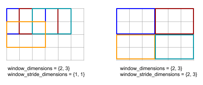
Basit olmayan bir dolgu örneği için 3 boyutuyla azaltılmış pencere minimum değerini (başlangıç değeri MAX_FLOAT) hesaplamayı ve [10000, 1000, 100, 10, 1] giriş dizisinin 2 boyunca ilerlemesini düşünün. kValid dolgusu, iki geçerli zaman aralığında minimum değerleri hesaplar: [10000, 1000, 100] ve [100, 10, 1], bu da [100, 1] çıkışı sağlar. kSame dolgusu, ilk olarak diziyi, azaltılmış pencereden sonraki şekil ile birinci adımın girişiyle aynı olacak şekilde doldurur. Bunun için her iki tarafa başlangıç öğeleri eklenerek [MAX_VALUE, 10000, 1000, 100, 10, 1,
MAX_VALUE] elde edilir. Dolgulu dizi üzerinde küçültme penceresi çalıştırma, üç pencerede ([MAX_VALUE, 10000, 1000], [1000, 100, 10], [10, 1, MAX_VALUE] ve getiri [1000, 10, 1]) çalışır.
İndirgeme işlevinin değerlendirme sırası isteğe bağlıdır ve belirli olmayabilir. Dolayısıyla, azaltma işlevi, yeniden ilişkilendirmeye aşırı duyarlı olmamalıdır. Daha ayrıntılı bilgi için Reduce bağlamında ilişkilendirme hakkındaki tartışmayı inceleyin.
ReplicaId
Ayrıca bkz.
XlaBuilder::ReplicaId.
Kopyanın benzersiz kimliğini (U32 skaler) döndürür.
ReplicaId()
Her replikanın benzersiz kimliği, [0, N) aralığındaki imzasız bir tam sayıdır. Burada N, replika sayısıdır. Tüm replikalar aynı programı çalıştırdığından, programdaki bir ReplicaId() çağrısı her replikada farklı bir değer döndürür.
Şekillendir
XlaBuilder::Reshape ve Collapse işlemini de inceleyin.
Bir dizinin boyutlarını yeni bir yapılandırmada yeniden şekillendirir.
Reshape(operand, new_sizes)
Reshape(operand, dimensions, new_sizes)
| Bağımsız değişkenler | Tür | Anlambilim |
|---|---|---|
operand |
XlaOp |
T türü dizisi |
dimensions |
int64 vektör |
boyutların daraltıldığı sırayla |
new_sizes |
int64 vektör |
yeni boyutlara sahip vektör |
Kavramsal olarak, yeniden şekillendirme ilk olarak bir diziyi veri değerlerinden oluşan tek boyutlu bir vektöre dönüştürür, ardından
bu vektörü yeni bir şekle sokar. Girdi bağımsız değişkenleri; T türünde rastgele bir dizi, boyut dizinlerinin derleme zamanı sabit vektörü ve sonuç için boyut boyutlarının derleme zaman sabit vektörüdür.
dimension vektöründeki değerler, sağlanmışsa tüm T boyutlarının permütasyonu olmalıdır; sağlanmazsa varsayılan değer {0, ..., rank - 1} olur. dimensions boyutundaki boyutların sırası, girdi dizisini tek bir boyuta daraltan döngü içindeki en yavaş değişen boyuttan (en büyük) en hızlı değişen boyuta (en küçük) doğrudur. new_sizes vektörü, çıkış dizisinin boyutunu belirler. new_sizes için dizin 0'daki değer 0 boyutun, dizin 1'deki değer 1'in boyutudur ve bu böyle devam eder. new_size boyutlarının çarpımı, işlenen boyut boyutlarının çarpımıyla eşit olmalıdır. Daraltılmış dizi, new_sizes tarafından tanımlanan çok boyutlu diziye daraltılırken new_sizes öğesindeki boyutlar en yavaş değişen (en büyük) ve en hızlı değişen (en küçük) doğru sıralanır.
Örneğin, v'nin 24 öğeli bir dizi olmasını sağlayın:
let v = f32[4x2x3] { { {10, 11, 12}, {15, 16, 17} },
                    { {20, 21, 22}, {25, 26, 27} },
                    { {30, 31, 32}, {35, 36, 37} },
                    { {40, 41, 42}, {45, 46, 47} } };

In-order collapse:
let v012_24 = Reshape(v, {0,1,2}, {24});
then v012_24 == f32[24] {10, 11, 12, 15, 16, 17, 20, 21, 22, 25, 26, 27,
                         30, 31, 32, 35, 36, 37, 40, 41, 42, 45, 46, 47};

let v012_83 = Reshape(v, {0,1,2}, {8,3});
then v012_83 == f32[8x3] { {10, 11, 12}, {15, 16, 17},
                          {20, 21, 22}, {25, 26, 27},
                          {30, 31, 32}, {35, 36, 37},
                          {40, 41, 42}, {45, 46, 47} };

Out-of-order collapse:
let v021_24 = Reshape(v, {1,2,0}, {24});
then v012_24 == f32[24]  {10, 20, 30, 40, 11, 21, 31, 41, 12, 22, 32, 42,
                          15, 25, 35, 45, 16, 26, 36, 46, 17, 27, 37, 47};

let v021_83 = Reshape(v, {1,2,0}, {8,3});
then v021_83 == f32[8x3] { {10, 20, 30}, {40, 11, 21},
                          {31, 41, 12}, {22, 32, 42},
                          {15, 25, 35}, {45, 16, 26},
                          {36, 46, 17}, {27, 37, 47} };


let v021_262 = Reshape(v, {1,2,0}, {2,6,2});
then v021_262 == f32[2x6x2] { { {10, 20}, {30, 40},
                              {11, 21}, {31, 41},
                              {12, 22}, {32, 42} },
                             { {15, 25}, {35, 45},
                              {16, 26}, {36, 46},
                              {17, 27}, {37, 47} } };
Özel bir durumda, yeniden şekillendirme işlemi tek öğeli bir diziyi skaler veya skaler diziye dönüştürebilir. Örneğin,
Reshape(f32[1x1] { {5} }, {0,1}, {}) == 5;
Reshape(5, {}, {1,1}) == f32[1x1] { {5} };
Gelir (ters)
Ayrıca bkz.
XlaBuilder::Rev.
Rev(operand, dimensions)
| Bağımsız değişkenler | Tür | Anlambilim |
|---|---|---|
operand |
XlaOp |
T türü dizisi |
dimensions |
ArraySlice<int64> |
tersine çevrilecek boyutlar |
Belirtilen dimensions boyunca operand dizisindeki öğelerin sırasını tersine çevirerek aynı şekilde bir çıkış dizisi oluşturur. Çok boyutlu dizindeki işlenen dizinin her bir öğesi, dönüştürülmüş bir dizindeki çıkış dizisinde depolanır. Çok boyutlu dizin, ters çevrilecek her bir boyuttaki dizinin tersine çevrilerek dönüştürülür (yani, N boyutu ters çeviren boyutlardan biriyse i dizini, N - 1 - i'ye dönüştürülür).
Rev işleminin bir kullanımı, nöral ağlardaki gradyan hesaplaması sırasında iki pencere boyutu boyunca evrişim ağırlık dizisini tersine çevirmektir.
RngNormal
Ayrıca bkz.
XlaBuilder::RngNormal.
Normal dağılımın ardından oluşturulan rastgele sayılarla belirli bir şeklin çıktısını \(N(\mu, \sigma)\) oluşturur. Parametreler \(\mu\) , \(\sigma\)ve çıkış şeklinin kayan nokta öğe türünde olması gerekir. Parametrelerin ek olarak skaler değerli olması gerekir.
RngNormal(mu, sigma, shape)
| Bağımsız değişkenler | Tür | Anlambilim |
|---|---|---|
mu |
XlaOp |
Oluşturulan sayıların ortalamasını belirten T türünde skaler |
sigma |
XlaOp |
Oluşturulan standart sapmayı belirten T türünde skaler |
shape |
Shape |
T tipi çıkış şekli |
RngUniform
Ayrıca bkz.
XlaBuilder::RngUniform.
Aralık boyunca tek tip dağılımın ardından oluşturulan rastgele sayılarla belirli bir şeklin çıktısını \([a,b)\)oluşturur. Parametrelerin ve çıkış öğesi türünün boole türünde, integral ya da kayan nokta türünde olması ve türlerin tutarlı olması gerekir. CPU ve GPU arka uçları şu anda yalnızca F64, F32, F16, BF16, S64, U64, S32 ve U32'yi desteklemektedir. Ayrıca, parametrelerin skaler değerli olması gerekir. Sonuç \(b <= a\) uygulama tanımlıysa.
RngUniform(a, b, shape)
| Bağımsız değişkenler | Tür | Anlambilim |
|---|---|---|
a |
XlaOp |
Aralık alt sınırını belirten T türünde skaler |
b |
XlaOp |
Aralık üst sınırını belirten T türünde skaler |
shape |
Shape |
T tipi çıkış şekli |
RngBitGenerator
Belirtilen algoritmayı (veya arka uç varsayılanını) kullanarak tek tip rastgele bitlerle dolu belirli bir şekille çıkış oluşturur ve güncellenmiş bir durumu (başlangıç durumuyla aynı şekilde) ve oluşturulan rastgele verileri döndürür.
Başlangıç durumu, geçerli rastgele sayı oluşturma işleminin ilk durumudur. Parametre değeri, gerekli şekil ve geçerli değerler, kullanılan algoritmaya bağlıdır.
Çıkışın, başlangıçtaki durumun belirleyici bir işlevi olacağı garanti edilir, ancak arka uçlar ve farklı derleyici sürümleri arasında belirleyici olacağı garanti edilmez.
RngBitGenerator(algorithm, key, shape)
| Bağımsız değişkenler | Tür | Anlambilim |
|---|---|---|
algorithm |
RandomAlgorithm |
PRNG algoritması kullanılır. |
initial_state |
XlaOp |
PRNG algoritması için başlangıç durumu. |
shape |
Shape |
Oluşturulan veriler için çıkış şekli. |
algorithm için kullanılabilir değerler:
rng_default: Arka uca özel şekil gereksinimleri olan arka uca özgü algoritma.rng_three_fry: ThreeFry sayacına dayalı PRNG algoritması.initial_stateşekli, rastgele değerlerleu64[2]şeklindedir. Salmon ve diğerleri SC 2011. Paralel rastgele sayılar: 1, 2, 3 gibi basit bir sayı kullanabilirsiniz.rng_philox: Paralel olarak rastgele sayılar oluşturan Philox algoritması.initial_stateşekli, rastgele değerlerleu64[3]şeklindedir. Salmon ve diğerleri SC 2011. Paralel rastgele sayılar: 1, 2, 3 gibi basit bir sayı kullanabilirsiniz.
Dağılım
XLA dağılım işlemi, operands giriş dizisinin değerleri olan bir sonuç dizisi oluşturur. Bazı dilimler (scatter_indices tarafından belirtilen dizinlerde), update_computation kullanılarak updates dilindeki değer dizisiyle güncellenir.
Ayrıca bkz.
XlaBuilder::Scatter.
scatter(operands..., scatter_indices, updates..., update_computation,
index_vector_dim, update_window_dims, inserted_window_dims,
scatter_dims_to_operand_dims)
| Bağımsız değişkenler | Tür | Anlambilim |
|---|---|---|
operands |
XlaOp. N dizisi |
Dağılım yapılacak N adet T_0, ..., T_N türü dizisi. |
scatter_indices |
XlaOp |
Dağılım alınması gereken dilimlerin başlangıç dizinlerini içeren dizi. |
updates |
XlaOp. N dizisi |
T_0, ..., T_N türünde N dizi. updates[i], operands[i] katmanını dağıtmak için kullanılması gereken değerleri içeriyor. |
update_computation |
XlaComputation |
Giriş dizisindeki mevcut değerleri ve dağılım sırasında güncellemeleri birleştirmek için kullanılacak hesaplama. Bu hesaplama T_0, ..., T_N, T_0, ..., T_N -> Collate(T_0, ..., T_N) türünde olmalıdır. |
index_vector_dim |
int64 |
scatter_indices politikasında, başlangıç dizinlerini içeren boyut. |
update_window_dims |
ArraySlice<int64> |
updates şeklinde, pencere boyutları olan boyut grubu. |
inserted_window_dims |
ArraySlice<int64> |
updates şekline eklenmesi gereken pencere boyutları grubu. |
scatter_dims_to_operand_dims |
ArraySlice<int64> |
Dağılım dizinlerinden işlenen dizin alanına boyutlar eşlemesi. Bu dizi, i ile scatter_dims_to_operand_dims[i] eşlemesi olarak yorumlanır . Bire bir ve toplam olmalıdır. |
indices_are_sorted |
bool |
Dizinlerin arayana göre sıralanmasının garanti edilip edilmediği. |
Burada:
- N, 1'den büyük veya 1'e eşit olmalıdır.
operands[0], ...,operands[N-1] aynı boyutlara sahip olmalıdır.updates[0], ...,updates[N-1] aynı boyutlara sahip olmalıdır.N = 1iseCollate(T),Tolur.N > 1iseCollate(T_0, ..., T_N),TtüründekiNöğelerinin bir demetidir.
index_vector_dim, scatter_indices.rank değerine eşitse dolaylı olarak scatter_indices öğesinin sonda bir 1 boyutu olduğunu düşünürüz.
ArraySlice<int64> türündeki update_scatter_dims, updates şeklinde, update_window_dims içinde olmayan, artan düzende boyut grubu olarak tanımlanır.
Dağılım bağımsız değişkenleri şu kısıtlamaları izlemelidir:
Her
updatesdizisiupdate_window_dims.size + scatter_indices.rank - 1sıralamasında olmalıdır.Her bir
updatesdizisindekiiboyutunun sınırları aşağıdakilere uygun olmalıdır:update_window_dimsiçindeivarsa (ör. bazıkiçinupdate_window_dims[k] değerine eşitse)updatesiçiniboyutunun sınırı,inserted_window_dimshesaba katıldıktan sonraoperanddeğerine karşılık gelen sınırı aşmamalıdır (ör.adjusted_window_bounds[k]; buradaadjusted_window_bounds, dizindeki sınırlar kaldırılmış olarakoperandsınırlarını içerir).inserted_window_dimsi,update_scatter_dimsiçinde mevcutsa (yani bazıkiçinupdate_scatter_dims[k] değerine eşitse)updatesiçindekiiboyutunun sınırı,index_vector_dimatlanarak karşılık gelenscatter_indicessınırına eşit olmalıdır (yanik<index_vector_dimisescatter_indices.shape.dims[k], aksi haldescatter_indices.shape.dims[k+1]).
update_window_dimsartan düzende olmalı, tekrarlanan boyut sayıları içermemelidir ve[0, updates.rank)aralığında olmalıdır.inserted_window_dimsartan düzende olmalı, tekrarlanan boyut sayıları içermemelidir ve[0, operand.rank)aralığında olmalıdır.operand.rank,update_window_dims.sizeileinserted_window_dims.sizetoplamına eşit olmalıdır.scatter_dims_to_operand_dims.size,scatter_indices.shape.dims[index_vector_dim] öğesine eşit olmalı ve değerleri[0, operand.rank)aralığında olmalıdır.
Her bir updates dizisindeki belirli bir U dizini için bu güncellemenin uygulanması gereken karşılık gelen operands dizisindeki karşılık gelen I dizini aşağıdaki gibi hesaplanır:
kiçinupdate_scatter_dims} konumundaG= {U[k] olsun.scatter_indicesdizisindeSindeks vektörünüSaramak içinS[i] =scatter_indices[Birleştir(G,i)] kullanın. Burada Birleştir(A; b),index_vector_dimkonumlarında b'yi A konumuna ekler.Gscatter_dims_to_operand_dimsharitasını kullanarakSöğelerini dağıtarakSkullanarakoperandiçinSindizini oluşturun. Daha resmî bir şekilde:k<scatter_dims_to_operand_dims.sizeiseSin[scatter_dims_to_operand_dims[k]] =S[k] olur.Sin[_] =0aksi takdirde.
Ubölgesindekiupdate_window_dimsdizinleriniinserted_window_dimsdoğrultusunda dağıtarak heroperandsdizisindeWindizininde bir dizin oluşturun. Daha resmî bir şekilde:Win[window_dims_to_operand_dims(k)] =U[k],kupdate_window_dimskonumundaysawindow_dims_to_operand_dims; alan [0,update_window_dims.size) ve [0,operand.rank) \inserted_window_dimsaralığına sahip monotonik fonksiyondur. (Örneğin,update_window_dims.size4,operand.rank6veinserted_window_dims{0,2} isewindow_dims_to_operand_dims{0→1,1→3,2→4,3→5} olur).Win[_] =0aksi takdirde.
I,Win+Sinşeklindedir. Burada +, öğe düzeyinde toplamadır.
Özetle, dağılım işlemi aşağıdaki gibi tanımlanabilir.
operands[J] dizisindeki tümOdizinleri içinoutputişleminioperandsile başlatın (ör. tüm dizinlerJiçin):
output[J][O] =operands[J][O]O,outputiçin geçerli bir dizinseupdates[J] dizisindeki herUdizini veoperand[J] dizisindeki karşılık gelenOdizini için:
(output[0][O], ...,output[N-1][O]) =update_computation(output[0][O], ..., ,output[N-1][O],updates[0][U], ...,updates[N-1][U])
Güncellemelerin uygulanma sırası belirleyici değildir. Dolayısıyla, updates içindeki birden fazla dizin operands dahilinde aynı dizine işaret ettiğinde, output içindeki karşılık gelen değer belirleyici olmaz.
update_computation öğesine iletilen ilk parametrenin her zaman output dizisindeki geçerli değer olacağını, ikinci parametrenin de her zaman updates dizisindeki değer olacağını unutmayın. Bu, özellikle update_computation değerinin değişkenli olmadığı durumlar için önemlidir.
indices_are_sorted doğru değerine ayarlanırsa XLA, start_indices öğesinin kullanıcı tarafından (artan start_index_map düzende) sıralandığını varsayabilir. Eşleşmezlerse anlamlar
uygulama olarak tanımlanır.
Gayriresmi olarak dağılım işlemi, toplama işleminin tersi olarak görülebilir. Diğer bir deyişle dağılım işlemi, girişteki ilgili toplama işlemi tarafından ayıklanan öğeleri günceller.
Resmi olmayan ayrıntılı açıklama ve örnekler için Gather altındaki "Resmi Olmayan Açıklama" bölümüne bakın.
Seçin
Ayrıca bkz.
XlaBuilder::Select.
Bir koşul dizisinin değerlerini temel alarak iki giriş dizisinin öğelerinden bir çıkış dizisi oluşturur.
Select(pred, on_true, on_false)
| Bağımsız değişkenler | Tür | Anlambilim |
|---|---|---|
pred |
XlaOp |
PRED türü dizisi |
on_true |
XlaOp |
T türü dizisi |
on_false |
XlaOp |
T türü dizisi |
on_true ve on_false dizileri aynı şekle sahip olmalıdır. Bu aynı zamanda çıkış dizisinin şeklidir. pred dizisi, PRED öğe türünde on_true ve on_false ile aynı boyuta sahip olmalıdır.
pred öğesinin her bir P öğesi için P değeri true ise çıkış dizisinin karşılık gelen öğesi on_true öğesinden alınır. P değeri true ise on_false öğesinden alınır.false Kısıtlanmış bir yayınlama biçimi olarak pred, PRED türünde skaler olabilir. Bu durumda, çıkış dizisi tamamen pred true ise on_true değerinden, pred false ise on_false değerinden alınır.
Skaler olmayan pred örneği:
let pred: PRED[4] = {true, false, false, true};
let v1: s32[4] = {1, 2, 3, 4};
let v2: s32[4] = {100, 200, 300, 400};
==>
Select(pred, v1, v2) = s32[4]{1, 200, 300, 4};
Skaler pred ile örnek:
let pred: PRED = true;
let v1: s32[4] = {1, 2, 3, 4};
let v2: s32[4] = {100, 200, 300, 400};
==>
Select(pred, v1, v2) = s32[4]{1, 2, 3, 4};
Tuple'lar arasında seçimler yapılabilir. Bu amaçla Tupler skaler tür olarak kabul edilir. on_true ve on_false de küçük kümelerse (aynı şekle sahip olmalıdır.) pred skaler PRED türünde olmalıdır.
SelectAndScatter
Ayrıca bkz.
XlaBuilder::SelectAndScatter.
Bu işlem, önce her pencereden bir öğe seçmek için operand dizisinde ReduceWindow hesaplaması yapan ve ardından işlenen diziyle aynı şekle sahip bir çıkış dizisi oluşturmak için source dizisini seçili öğelerin dizinlerine dağıtan birleşik bir işlem olarak düşünülebilir. İkili select işlevi, öğeyi her bir pencereye uygulayarak her pencereden bir öğe seçmek için kullanılır ve ilk parametrenin dizin vektörünün, sözlük açısından ikinci parametrenin dizin vektöründen daha küçük olması özelliğiyle çağrılır. select işlevi, birinci parametre seçilirse true değerini, ikinci parametre seçilirse false değerini döndürür ve seçilen öğenin belirli bir pencerede geçirilen öğelerin sırasına bağlı olmaması için işlevin geçişliliği koruması (ör. select(a, b) ve select(b, c) ise true ise select(a, c) de true olur) gerekir.
scatter işlevi, çıkış dizisinde seçilen her dizine uygulanır. İki skaler parametre alır:
- Çıkış dizisinde seçili dizindeki geçerli değer
- Seçili dizine uygulanan
sourcedağılım değeri
İki parametreyi birleştirir ve çıkış dizisinde, seçilen dizindeki değeri güncellemek için kullanılan skaler bir değer döndürür. Başlangıçta, çıkış dizisinin tüm dizinleri init_value olarak ayarlanır.
Çıkış dizisi, operand dizisiyle aynı şekle sahip olmalıdır ve source dizisi, operand dizisine ReduceWindow işlemi uygulanmasının sonucuyla aynı şekle sahip olmalıdır. SelectAndScatter, nöral ağdaki bir havuz katmanına ilişkin gradyan değerlerini geriye yaymak için kullanılabilir.
SelectAndScatter(operand, select, window_dimensions, window_strides,
padding, source, init_value, scatter)
| Bağımsız değişkenler | Tür | Anlambilim |
|---|---|---|
operand |
XlaOp |
pencerelerin üzerinden kaydırıldığı T türü dizisi |
select |
XlaComputation |
her bir penceredeki tüm öğelere uygulanacak T, T -> PRED türünde ikili hesaplama; ilk parametre seçilirse true ve ikinci parametre seçilirse false döndürülür |
window_dimensions |
ArraySlice<int64> |
pencere boyutu değerleri için tam sayı dizisi |
window_strides |
ArraySlice<int64> |
pencere adımı değerleri için tam sayı dizisi |
padding |
Padding |
pencere için dolgu türü (Dolgu::kSame veya Dolgu::kValid) |
source |
XlaOp |
dağıtılacak değerleri içeren T türü dizi |
init_value |
XlaOp |
çıkış dizisinin başlangıç değeri için T türünün skaler değeri |
scatter |
XlaComputation |
Her dağılım kaynağı öğesini hedef öğesiyle uygulamak için T, T -> T türünde ikili hesaplama |
Aşağıdaki şekilde, select işlevinin parametreleri arasında maksimum değeri hesapladığı SelectAndScatter kullanımına ilişkin örnekler gösterilmektedir. Pencereler çakıştığında, aşağıdaki şekilde (2) gösterildiği gibi, operand dizisinin bir dizininin farklı pencereler tarafından birden fazla kez seçilebileceğini unutmayın. Şekilde, 9 değerinin öğesi hem üstteki pencereler (mavi ve kırmızı) tarafından seçilmiş hem de ikili toplama scatter işlevi 8 değerinin çıktı öğesini (2 + 6) verir.
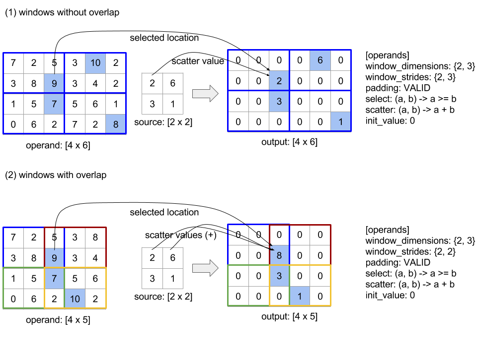
scatter işlevinin değerlendirme sırası rastgeledir ve belirleyici olmayabilir. Bu nedenle, scatter işlevi yeniden ilişkilendirmeye karşı aşırı hassas olmamalıdır. Daha ayrıntılı bilgi için Reduce bağlamında ilişkilendirme hakkındaki tartışmayı inceleyin.
Gönder
Ayrıca bkz.
XlaBuilder::Send.
Send(operand, channel_handle)
| Bağımsız değişkenler | Tür | Anlambilim |
|---|---|---|
operand |
XlaOp |
gönderilecek veriler (T türündeki dizi) |
channel_handle |
ChannelHandle |
her gönder/al çifti için benzersiz tanımlayıcı |
Belirtilen işlenen verileri, aynı kanal işleyiciyi paylaşan başka bir hesaplamadaki Recv talimatına gönderir. Veri döndürmez.
Recv işlemine benzer şekilde, Send işleminin istemci API'si eşzamanlı iletişimi temsil eder ve eşzamansız veri aktarımlarını etkinleştirmek için 2 HLO talimatına (Send ve SendDone) ayrılmıştır. Ayrıca bkz.
HloInstruction::CreateSend ve HloInstruction::CreateSendDone.
Send(HloInstruction operand, int64 channel_id)
İşlenenin, Recv talimatı tarafından aynı kanal kimliğine sahip olan kaynaklara eşzamansız bir şekilde aktarılmasını başlatır. Veri aktarımının tamamlanmasını beklemek için aşağıdaki SendDone talimatı tarafından kullanılan bir bağlam döndürür. Bağlam, bir {operand (shape), istek tanımlayıcısı (U32)} unsurudur ve yalnızca bir SendDone talimatı tarafından kullanılabilir.
SendDone(HloInstruction context)
Send talimatıyla oluşturulan bir bağlamda veri aktarımının tamamlanmasını bekler. Talimat herhangi bir veri döndürmez.
Kanal talimatlarını planlama
Her kanal için (Recv, RecvDone,
Send, SendDone) 4 talimatın uygulanma sırası aşağıdaki gibidir.
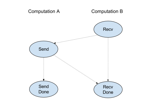
Recv,Sendtarihinden önce gerçekleşirSend,RecvDonetarihinden önce gerçekleşirRecv,RecvDonetarihinden önce gerçekleşirSend,SendDonetarihinden önce gerçekleşir
Arka uç derleyicileri, kanal talimatları aracılığıyla iletişim kuran her hesaplama için doğrusal bir program oluşturduğunda hesaplamalar arasında döngü olmaması gerekir. Örneğin, aşağıdaki programlar kilitlenmelere yol açabilir.
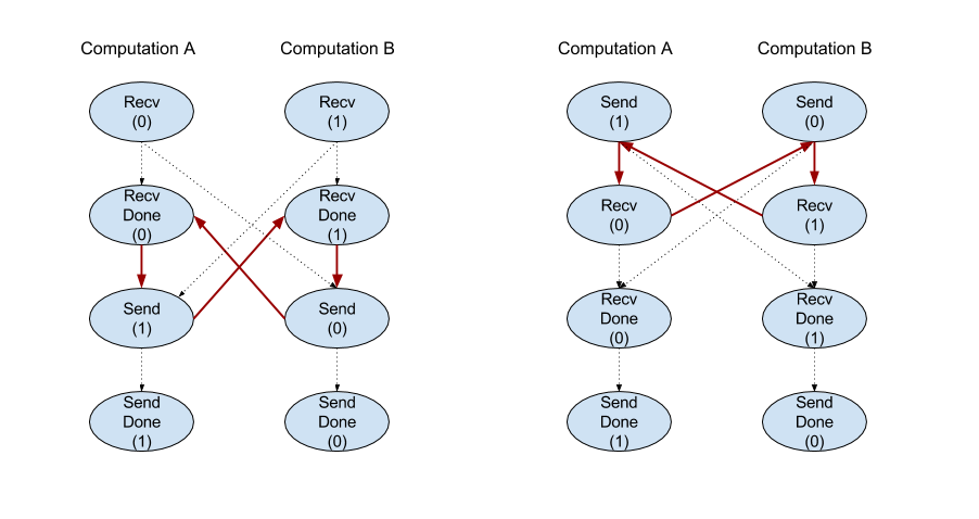
Dilim
Ayrıca bkz.
XlaBuilder::Slice.
Dilimleme işlemi, giriş dizisinden bir alt dizi çıkarır. Alt dizi, girişle aynı sıralamaya sahiptir ve değerleri, giriş dizisindeki bir sınırlayıcı kutunun içinde içerir. Sınırlayıcı kutunun boyutları ve dizinleri, dilim işlemi için bağımsız değişkenler olarak verilir.
Slice(operand, start_indices, limit_indices, strides)
| Bağımsız değişkenler | Tür | Anlambilim |
|---|---|---|
operand |
XlaOp |
T türünde N boyutlu dizi |
start_indices |
ArraySlice<int64> |
Her boyut için dilimin başlangıç dizinlerini içeren N tam sayıdan oluşan liste. Değerler sıfırdan büyük veya sıfıra eşit olmalıdır. |
limit_indices |
ArraySlice<int64> |
Her boyuta ait dilimin bitiş dizinlerini (hariç) içeren N tam sayıdan oluşan liste. Her değer, boyutun ilgili start_indices değerinden büyük ya da bu değere eşit ve boyutun boyutundan küçük ya da bu değere eşit olmalıdır. |
strides |
ArraySlice<int64> |
Dilimin giriş adımını belirleyen N tam sayıdan oluşan liste. Dilim, d boyutundaki her strides[d] öğesini seçer. |
1 boyutlu örnek:
let a = {0.0, 1.0, 2.0, 3.0, 4.0}
Slice(a, {2}, {4}) produces:
  {2.0, 3.0}
2 boyutlu örnek:
let b =
 { {0.0,  1.0,  2.0},
   {3.0,  4.0,  5.0},
   {6.0,  7.0,  8.0},
   {9.0, 10.0, 11.0} }

Slice(b, {2, 1}, {4, 3}) produces:
  { { 7.0,  8.0},
    {10.0, 11.0} }
Sırala
Ayrıca bkz.
XlaBuilder::Sort.
Sort(operands, comparator, dimension, is_stable)
| Bağımsız değişkenler | Tür | Anlambilim |
|---|---|---|
operands |
ArraySlice<XlaOp> |
Sıralanacak işlenenler. |
comparator |
XlaComputation |
Kullanılacak karşılaştırıcı hesaplaması. |
dimension |
int64 |
Sıralama için kullanılacak boyut. |
is_stable |
bool |
Sabit sıralamanın kullanılıp kullanılmayacağı. |
Yalnızca bir işlenen sağlanırsa:
İşlem gören bir sıra 1 tensörü (dizi) ise sonuç sıralı bir dizidir. Diziyi artan düzende sıralamak istiyorsanız karşılaştırıcı, "daha düşük" bir karşılaştırma yapmalıdır. Resmî olarak, dizi sıralandıktan sonra
comparator(value[i], value[j]) = comparator(value[j], value[i]) = falseveyacomparator(value[i], value[j]) = trueolani < jiçeren tüm dizin konumlarını içerir.i, jİşlem gören daha yüksek bir sıralamaya sahipse işlenen boyut, sağlanan boyut boyunca sıralanır. Örneğin, bir sıra 2 tensörü (matris) için
0boyut değeri her sütunu bağımsız olarak sıralar ve1boyut değeri her bir satırı bağımsız olarak sıralar. Herhangi bir boyut numarası sağlanmazsa varsayılan olarak son boyut seçilir. Sıralanan boyut için rank-1 örneğindekiyle aynı sıralama düzeni geçerlidir.
n > 1 işlenenler sağlanırsa:
Tüm
nişlenenleri, aynı boyutlara sahip tensörler olmalıdır. Tensörlerin eleman türleri farklı olabilir.Tüm işlenenler tek tek değil birlikte sıralanır. Kavramsal olarak işlenenler, tuple kabul edilir.
ivejdizin konumlarındaki her bir işlenene ait öğelerin değiştirilmesinin gerekip gerekmediğini kontrol ederken, karşılaştırıcı2 * nskaler parametrelerle çağrılır. Burada2 * kparametresi,k-thişlenenindenikonumundakiikonumundaki değere,2 * k + 1parametresi dek-thişlenenindenjkonumundaki değere karşılık gelir. Bu durumda karşılaştırıcı, genellikle2 * kve2 * k + 1parametrelerini birbirleriyle karşılaştırır ve bağlantı kesici olarak başka parametre çiftlerini kullanır.Sonuç, sıralanmış sırada (yukarıda olduğu gibi sağlanan boyutla birlikte) işlenenlerden oluşan bir unsurdur. Tuple'ın
i-thişleneni, Sort'uni-thişlenenine karşılık gelir.
Örneğin, üç işlenen operand0 = [3, 1], operand1 = [42, 50], operand2 = [-3.0, 1.1] varsa ve karşılaştırıcı yalnızca operand0 değerlerini küçüktür ile karşılaştırıyorsa sıralama çıktısı ([1, 3], [50, 42], [1.1, -3.0]) demeti olur.
is_stable doğru değerine ayarlanırsa sıralamanın kararlı olacağı garanti edilir. Diğer bir deyişle, karşılaştırıcı tarafından eşit olarak kabul edilen öğeler varsa eşit değerlerin göreli sıralaması korunur. e1 ve e2 iki öğe, yalnızca comparator(e1, e2) = comparator(e2, e1) = false ise eşittir. is_stable varsayılan olarak "false" değerine ayarlanmıştır.
Ters çevirme
Ayrıca tf.reshape işlemine de bakın.
Transpose(operand)
| Bağımsız değişkenler | Tür | Anlambilim |
|---|---|---|
operand |
XlaOp |
Ters çevrilmiştir. |
permutation |
ArraySlice<int64> |
Boyutlara nasıl permütasyon yapılır? |
Belirtilen permütasyonla işlenen boyutlara permütasyon yapar. Dolayısıyla ∀ i . 0 ≤ i < rank ⇒ input_dimensions[permutation[i]] = output_dimensions[i].
Bu işlem, Yeniden Şekillendirme(işleme alınan, permütasyon, Permüt(permütasyon, işlenen.şekil.boyutlar)) ile aynıdır.
TriangularSolve
Ayrıca bkz.
XlaBuilder::TriangularSolve.
Alt veya üst üçgen katsayı matrisleri içeren doğrusal denklem sistemlerini ileri ya da geri yerine koyma yöntemiyle çözer. Öncü boyutlarla yayın yapan bu rutin, a ve b değişkeni için x değişkeni için op(a) * x =
b veya x * op(a) = b matris sistemlerinden birini çözer. Burada op(a) op(a) = a veya op(a) = Transpose(a) ya da op(a) = Conj(Transpose(a)) olur.
TriangularSolve(a, b, left_side, lower, unit_diagonal, transpose_a)
| Bağımsız değişkenler | Tür | Anlambilim |
|---|---|---|
a |
XlaOp |
[..., M, M] şeklinde karmaşık veya kayan nokta türünde sıralamadan en az 2 dizi. |
b |
XlaOp |
left_side doğruysa [..., M, K] şekline sahip aynı türde > 2 dizi, doğru değilse [..., K, M]. |
left_side |
bool |
bir sistemin op(a) * x = b (true) veya x * op(a) = b (false) biçiminde mi çözülmesi gerektiğini gösterir. |
lower |
bool |
a öğesinin üst veya alt üçgenini kullanıp kullanmayacağınızı belirleyin. |
unit_diagonal |
bool |
true ise a öğesinin köşegen öğelerinin 1 olduğu varsayılır ve bu öğelere erişilmez. |
transpose_a |
Transpose |
a öğesinin olduğu gibi kullanılıp kullanılmayacağını, ters çevirin veya eşlenik ters çevirmenin yapılıp yapılmayacağını belirleyin. |
Giriş verileri, lower değerine bağlı olarak yalnızca a alt/üst üçgeninden okunur. Diğer üçgendeki değerler yoksayılır. Çıktı verileri aynı üçgen içinde döndürülür; diğer üçgendeki değerler uygulama tanımlıdır ve herhangi bir değer olabilir.
a ve b sıralaması 2'den büyükse bunlar matris grupları olarak ele alınır. Küçük 2 boyut dışındaki tüm boyutlar grup boyutlarıdır. a ve
b eşit grup boyutlarına sahip olmalıdır.
Tuple
Ayrıca bkz.
XlaBuilder::Tuple.
Değişken sayıda veri işleyicisi içeren ve her birinin kendi şekli olan bir unsur.
Bu, C++'taki std::tuple yönergesine benzer. Kavramsal olarak:
let v: f32[10] = f32[10]{0, 1, 2, 3, 4, 5, 6, 7, 8, 9};
let s: s32 = 5;
let t: (f32[10], s32) = tuple(v, s);
Tuple'lar, GetTupleElement işlemi aracılığıyla ayrıştırılabilir (erişilebilir).
Kullanım
Ayrıca bkz.
XlaBuilder::While.
While(condition, body, init)
| Bağımsız değişkenler | Tür | Anlambilim |
|---|---|---|
condition |
XlaComputation |
Döngünün sonlandırma koşulunu tanımlayan T -> PRED türündeki XlaComputation. |
body |
XlaComputation |
Döngünün gövdesini tanımlayan T -> T türündeki XlaComputation. |
init |
T |
condition ve body parametresi için başlangıç değeri. |
condition başarısız olana kadar body öğesini sırayla yürütür. Bu, aşağıda listelenen farklılıklar ve kısıtlamalar dışında diğer birçok dilde gerçekleşen tipik bir döngüye benzer.
Whiledüğümü,Ttüründe bir değer döndürür. Bu,bodyişleminin son yürütmesinin sonucudur.Ttürünün şekli statik olarak belirlenir ve tüm yinelemelerde aynı olmalıdır.
Hesaplamaların T parametreleri, ilk iterasyonda init değeriyle başlatılır ve sonraki her yinelemede body parametresinden elde edilen yeni sonuca otomatik olarak güncellenir.
While düğümünün ana kullanım alanlarından biri, nöral ağlarda eğitimin tekrar eden yürütülmesini uygulamaktır. Basitleştirilmiş sözde kod, hesaplamayı temsil eden bir grafikle birlikte aşağıda gösterilmektedir. Kodu while_test.cc adresinde bulabilirsiniz.
Bu örnekteki T türü, yineleme sayısı için int32 ve toplayıcı için vector[10] içeren bir Tuple'dir. 1000 yinelemede döngü, toplayıcıya sabit bir vektör eklemeye devam eder.
// Pseudocode for the computation.
init = {0, zero_vector[10]} // Tuple of int32 and float[10].
result = init;
while (result(0) < 1000) {
  iteration = result(0) + 1;
  new_vector = result(1) + constant_vector[10];
  result = {iteration, new_vector};
}