
|
|
|
 View on GitHub View on GitHub
|
|
Welcome to the Learning to Rank Colab for TensorFlow Decision Forests (TF-DF). In this colab, you will learn how to use TF-DF for ranking.
This colab assumes you are familiar with the concepts presented the Beginner colab, notably about the installation about TF-DF.
In this colab, you will:
- Learn what a ranking model is.
- Train a Gradient Boosted Trees models on the LETOR3 dataset.
- Evaluate the quality of this model.
Installing TensorFlow Decision Forests
Install TF-DF by running the following cell.
pip install tensorflow_decision_forestsWurlitzer is needed to display the detailed training logs in Colabs (when using verbose=2 in the model constructor).
pip install wurlitzerImporting libraries
import os
# Keep using Keras 2
os.environ['TF_USE_LEGACY_KERAS'] = '1'

import tensorflow_decision_forests as tfdf

import numpy as np
import pandas as pd
import tensorflow as tf
import tf_keras
import math
2025-03-10 11:10:00.213521: E external/local_xla/xla/stream_executor/cuda/cuda_fft.cc:477] Unable to register cuFFT factory: Attempting to register factory for plugin cuFFT when one has already been registered
WARNING: All log messages before absl::InitializeLog() is called are written to STDERR
E0000 00:00:1741605000.234714    9343 cuda_dnn.cc:8310] Unable to register cuDNN factory: Attempting to register factory for plugin cuDNN when one has already been registered
E0000 00:00:1741605000.241231    9343 cuda_blas.cc:1418] Unable to register cuBLAS factory: Attempting to register factory for plugin cuBLAS when one has already been registered
The hidden code cell limits the output height in colab.
from IPython.core.magic import register_line_magic
from IPython.display import Javascript
from IPython.display import display as ipy_display

# Some of the model training logs can cover the full
# screen if not compressed to a smaller viewport.
# This magic allows setting a max height for a cell.
@register_line_magic
def set_cell_height(size):
  ipy_display(
      Javascript("google.colab.output.setIframeHeight(0, true, {maxHeight: " +
                 str(size) + "})"))
# Check the version of TensorFlow Decision Forests
print("Found TensorFlow Decision Forests v" + tfdf.__version__)
Found TensorFlow Decision Forests v1.11.0
What is a ranking model?
The goal of a ranking model is to correctly order items. For example, ranking can be used to select the best documents to retrieve following a user query.
A common way to represent a Ranking dataset is with a "relevance" score: The order of the elements is defined by their relevance: Items of greater relevance should be before lower relevance items. The cost of a mistake is defined by the difference between the relevance of the predicted item with the relevance of the correct item. For example, misordering two items with respective relevance 3 and 4 is not as bad as misordering two items with respective relevance 1 and 5.
TF-DF expects ranking datasets to be presented in a "flat" format. A dataset of queries and corresponding documents might look like this:
| query | document_id | feature_1 | feature_2 | relevance |
|---|---|---|---|---|
| cat | 1 | 0.1 | blue | 4 |
| cat | 2 | 0.5 | green | 1 |
| cat | 3 | 0.2 | red | 2 |
| dog | 4 | NA | red | 0 |
| dog | 5 | 0.2 | red | 0 |
| dog | 6 | 0.6 | green | 1 |
The relevance/label is a floating point numerical value between 0 and 5 (generally between 0 and 4) where 0 means "completely unrelated", 4 means "very relevant" and 5 means "same as the query".
In this example, Document 1 is very relevant to the query "cat", while document 2 is only "related" to cats. There are no documents is really talking about "dog" (the highest relevance is 1 for the document 6). However, the dog query is still expecting to return document 6 (since this is the document that talks the "most" about dogs).
Interestingly, decision forests are often good rankers, and many state-of-the-art ranking models are decision forests.
Let's train a Ranking model
In this example, use a sample of the
LETOR3
dataset. More precisely, we want to download the OHSUMED.zip from the LETOR3 repo. This dataset is stored in the
libsvm format, so we will need to convert it to csv.
archive_path = tf_keras.utils.get_file("letor.zip",
  "https://download.microsoft.com/download/E/7/E/E7EABEF1-4C7B-4E31-ACE5-73927950ED5E/Letor.zip",
  extract=True)

# Path to a ranking ataset using libsvm format.
raw_dataset_path = os.path.join(os.path.dirname(archive_path),"OHSUMED/Data/Fold1/trainingset.txt")
Downloading data from https://download.microsoft.com/download/E/7/E/E7EABEF1-4C7B-4E31-ACE5-73927950ED5E/Letor.zip
61824018/61824018 [==============================] - 1s 0us/step
Here are the first lines of the dataset:
head {raw_dataset_path}The first step is to convert this dataset to the "flat" format mentioned above.
def convert_libsvm_to_csv(src_path, dst_path):
  """Converts a libsvm ranking dataset into a flat csv file.

  Note: This code is specific to the LETOR3 dataset.
  """
  dst_handle = open(dst_path, "w")
  first_line = True
  for src_line in open(src_path,"r"):
    # Note: The last 3 items are comments.
    items = src_line.split(" ")[:-3]
    relevance = items[0]
    group = items[1].split(":")[1]
    features = [ item.split(":") for item in items[2:]]

    if first_line:
      # Csv header
      dst_handle.write("relevance,group," + ",".join(["f_" + feature[0] for feature in features]) + "\n")
      first_line = False
    dst_handle.write(relevance + ",g_" + group + "," + (",".join([feature[1] for feature in features])) + "\n")
  dst_handle.close()

# Convert the dataset.
csv_dataset_path="/tmp/ohsumed.csv"
convert_libsvm_to_csv(raw_dataset_path, csv_dataset_path)

# Load a dataset into a Pandas Dataframe.
dataset_df = pd.read_csv(csv_dataset_path)

# Display the first 3 examples.
dataset_df.head(3)
In this dataset, each row represents a pair of query/document (called "group"). The "relevance" tells how much the query matches the document.
The features of the query and the document are merged together in "f1-25". The exact definition of the features is not known, but it would be something like:
- Number of words in queries
- Number of common words between the query and the document
- Cosinus similarity between an embedding of the query and an embedding of the document.
- ...
Let's convert the Pandas Dataframe into a TensorFlow Dataset:
dataset_ds = tfdf.keras.pd_dataframe_to_tf_dataset(dataset_df, label="relevance", task=tfdf.keras.Task.RANKING)
I0000 00:00:1741605007.271607    9343 gpu_device.cc:2022] Created device /job:localhost/replica:0/task:0/device:GPU:0 with 13638 MB memory:  -> device: 0, name: Tesla T4, pci bus id: 0000:00:05.0, compute capability: 7.5
I0000 00:00:1741605007.273751    9343 gpu_device.cc:2022] Created device /job:localhost/replica:0/task:0/device:GPU:1 with 13756 MB memory:  -> device: 1, name: Tesla T4, pci bus id: 0000:00:06.0, compute capability: 7.5
I0000 00:00:1741605007.275787    9343 gpu_device.cc:2022] Created device /job:localhost/replica:0/task:0/device:GPU:2 with 13756 MB memory:  -> device: 2, name: Tesla T4, pci bus id: 0000:00:07.0, compute capability: 7.5
I0000 00:00:1741605007.277920    9343 gpu_device.cc:2022] Created device /job:localhost/replica:0/task:0/device:GPU:3 with 13756 MB memory:  -> device: 3, name: Tesla T4, pci bus id: 0000:00:08.0, compute capability: 7.5
Let's configure and train our Ranking model.
%set_cell_height 400

model = tfdf.keras.GradientBoostedTreesModel(
    task=tfdf.keras.Task.RANKING,
    ranking_group="group",
    num_trees=50)

model.fit(dataset_ds)
<IPython.core.display.Javascript object>
Warning: The `num_threads` constructor argument is not set and the number of CPU is os.cpu_count()=32 > 32. Setting num_threads to 32. Set num_threads manually to use more than 32 cpus.
WARNING:absl:The `num_threads` constructor argument is not set and the number of CPU is os.cpu_count()=32 > 32. Setting num_threads to 32. Set num_threads manually to use more than 32 cpus.
Use /tmpfs/tmp/tmp3c_k9qah as temporary training directory
Reading training dataset...
2025-03-10 11:10:07.650348: W external/ydf/yggdrasil_decision_forests/learner/gradient_boosted_trees/gradient_boosted_trees.cc:1840] "goss_alpha" set but "sampling_method" not equal to "GOSS".
2025-03-10 11:10:07.650382: W external/ydf/yggdrasil_decision_forests/learner/gradient_boosted_trees/gradient_boosted_trees.cc:1850] "goss_beta" set but "sampling_method" not equal to "GOSS".
2025-03-10 11:10:07.650389: W external/ydf/yggdrasil_decision_forests/learner/gradient_boosted_trees/gradient_boosted_trees.cc:1864] "selective_gradient_boosting_ratio" set but "sampling_method" not equal to "SELGB".
Training dataset read in 0:00:04.014234. Found 9219 examples.
Training model...
WARNING: All log messages before absl::InitializeLog() is called are written to STDERR
I0000 00:00:1741605011.690068    9343 kernel.cc:782] Start Yggdrasil model training
I0000 00:00:1741605011.690125    9343 kernel.cc:783] Collect training examples
I0000 00:00:1741605011.690132    9343 kernel.cc:795] Dataspec guide:
column_guides {
  column_name_pattern: "^__LABEL$"
  type: NUMERICAL
}
default_column_guide {
  categorial {
    max_vocab_count: 2000
  }
  discretized_numerical {
    maximum_num_bins: 255
  }
}
ignore_columns_without_guides: false
detect_numerical_as_discretized_numerical: false

I0000 00:00:1741605011.690499    9343 kernel.cc:401] Number of batches: 10
I0000 00:00:1741605011.690512    9343 kernel.cc:402] Number of examples: 9219
I0000 00:00:1741605011.692259    9343 kernel.cc:802] Training dataset:
Number of records: 9219
Number of columns: 27

Number of columns by type:
    NUMERICAL: 26 (96.2963%)
    HASH: 1 (3.7037%)

Columns:

NUMERICAL: 26 (96.2963%)
    0: "__LABEL" NUMERICAL mean:0.495607 min:0 max:2 sd:0.744403
    1: "f_1" NUMERICAL mean:1.21141 min:0 max:7 sd:1.15164
    2: "f_10" NUMERICAL mean:4.20167 min:0 max:21.0369 sd:3.88154
    3: "f_11" NUMERICAL mean:4.33312 min:0 max:59 sd:4.67348
    4: "f_12" NUMERICAL mean:1.91775 min:0 max:9.75731 sd:1.61639
    5: "f_13" NUMERICAL mean:0.0457776 min:0 max:0.384615 sd:0.0466109
    6: "f_14" NUMERICAL mean:0.0447853 min:0 max:0.361682 sd:0.0451178
    7: "f_15" NUMERICAL mean:21.3512 min:11.4845 max:39.1502 sd:6.03344
    8: "f_16" NUMERICAL mean:6.70697 min:3.95484 max:12.369 sd:1.80357
    9: "f_17" NUMERICAL mean:19.534 min:10.2355 max:40.1808 sd:6.08569
    10: "f_18" NUMERICAL mean:0.195288 min:0 max:1.3212 sd:0.187686
    11: "f_19" NUMERICAL mean:20.1237 min:0 max:176.805 sd:20.9556
    12: "f_2" NUMERICAL mean:0.825689 min:0 max:4.27667 sd:0.772347
    13: "f_20" NUMERICAL mean:1.8782 min:0 max:11.6585 sd:1.75127
    14: "f_21" NUMERICAL mean:12.2408 min:3.18098 max:45.0899 sd:6.76927
    15: "f_22" NUMERICAL mean:2.31505 min:1.15719 max:3.80866 sd:0.666958
    16: "f_23" NUMERICAL mean:-6.0857 min:-9.49097 max:-1.85651 sd:2.13886
    17: "f_24" NUMERICAL mean:-5.83816 min:-9.22971 max:-1.02685 sd:1.96046
    18: "f_25" NUMERICAL mean:-5.98972 min:-9.60073 max:-1.02685 sd:2.16203
    19: "f_3" NUMERICAL mean:0.161865 min:0 max:1 sd:0.165642
    20: "f_4" NUMERICAL mean:0.149731 min:0 max:0.892574 sd:0.149804
    21: "f_5" NUMERICAL mean:26.3233 min:15.3432 max:51.3862 sd:7.40231
    22: "f_6" NUMERICAL mean:7.82971 min:4.24645 max:15.3248 sd:2.09136
    23: "f_7" NUMERICAL mean:26.9268 min:15.3265 max:52.0258 sd:8.07986
    24: "f_8" NUMERICAL mean:0.64629 min:0 max:3.59024 sd:0.614985
    25: "f_9" NUMERICAL mean:6.78251 min:0 max:47.7046 sd:6.26551

HASH: 1 (3.7037%)
    26: "group" HASH

Terminology:
    nas: Number of non-available (i.e. missing) values.
    ood: Out of dictionary.
    manually-defined: Attribute whose type is manually defined by the user, i.e., the type was not automatically inferred.
    tokenized: The attribute value is obtained through tokenization.
    has-dict: The attribute is attached to a string dictionary e.g. a categorical attribute stored as a string.
    vocab-size: Number of unique values.

I0000 00:00:1741605011.692302    9343 kernel.cc:818] Configure learner
2025-03-10 11:10:11.692565: W external/ydf/yggdrasil_decision_forests/learner/gradient_boosted_trees/gradient_boosted_trees.cc:1840] "goss_alpha" set but "sampling_method" not equal to "GOSS".
2025-03-10 11:10:11.692599: W external/ydf/yggdrasil_decision_forests/learner/gradient_boosted_trees/gradient_boosted_trees.cc:1850] "goss_beta" set but "sampling_method" not equal to "GOSS".
2025-03-10 11:10:11.692608: W external/ydf/yggdrasil_decision_forests/learner/gradient_boosted_trees/gradient_boosted_trees.cc:1864] "selective_gradient_boosting_ratio" set but "sampling_method" not equal to "SELGB".
I0000 00:00:1741605011.692654    9343 kernel.cc:831] Training config:
learner: "GRADIENT_BOOSTED_TREES"
features: "^f_1$"
features: "^f_10$"
features: "^f_11$"
features: "^f_12$"
features: "^f_13$"
features: "^f_14$"
features: "^f_15$"
features: "^f_16$"
features: "^f_17$"
features: "^f_18$"
features: "^f_19$"
features: "^f_2$"
features: "^f_20$"
features: "^f_21$"
features: "^f_22$"
features: "^f_23$"
features: "^f_24$"
features: "^f_25$"
features: "^f_3$"
features: "^f_4$"
features: "^f_5$"
features: "^f_6$"
features: "^f_7$"
features: "^f_8$"
features: "^f_9$"
label: "^__LABEL$"
task: RANKING
random_seed: 123456
ranking_group: "group"
metadata {
  framework: "TF Keras"
}
pure_serving_model: false
[yggdrasil_decision_forests.model.gradient_boosted_trees.proto.gradient_boosted_trees_config] {
  num_trees: 50
  decision_tree {
    max_depth: 6
    min_examples: 5
    in_split_min_examples_check: true
    keep_non_leaf_label_distribution: true
    num_candidate_attributes: -1
    missing_value_policy: GLOBAL_IMPUTATION
    allow_na_conditions: false
    categorical_set_greedy_forward {
      sampling: 0.1
      max_num_items: -1
      min_item_frequency: 1
    }
    growing_strategy_local {
    }
    categorical {
      cart {
      }
    }
    axis_aligned_split {
    }
    internal {
      sorting_strategy: PRESORTED
    }
    uplift {
      min_examples_in_treatment: 5
      split_score: KULLBACK_LEIBLER
    }
  }
  shrinkage: 0.1
  loss: DEFAULT
  validation_set_ratio: 0.1
  validation_interval_in_trees: 1
  early_stopping: VALIDATION_LOSS_INCREASE
  early_stopping_num_trees_look_ahead: 30
  l2_regularization: 0
  lambda_loss: 1
  mart {
  }
  adapt_subsample_for_maximum_training_duration: false
  l1_regularization: 0
  use_hessian_gain: false
  l2_regularization_categorical: 1
  xe_ndcg {
    ndcg_truncation: 5
  }
  stochastic_gradient_boosting {
    ratio: 1
  }
  apply_link_function: true
  compute_permutation_variable_importance: false
  early_stopping_initial_iteration: 10
}

I0000 00:00:1741605011.693006    9343 kernel.cc:834] Deployment config:
cache_path: "/tmpfs/tmp/tmp3c_k9qah/working_cache"
num_threads: 32
try_resume_training: true

I0000 00:00:1741605011.693195    9568 kernel.cc:895] Train model
I0000 00:00:1741605011.695548    9568 loss_interface.cc:139] Found 58 groups in 8365 examples.
I0000 00:00:1741605011.695618    9568 loss_interface.cc:139] Found 5 groups in 854 examples.
Model trained in 0:00:00.576673
Compiling model...
I0000 00:00:1741605012.245982    9568 early_stopping.cc:54] Early stop of the training because the validation loss does not decrease anymore. Best valid-loss: -0.438692
I0000 00:00:1741605012.247742    9568 kernel.cc:926] Export model in log directory: /tmpfs/tmp/tmp3c_k9qah with prefix 9a0bfc5f657b4150
I0000 00:00:1741605012.248195    9568 kernel.cc:944] Save model in resources
I0000 00:00:1741605012.251748    9343 abstract_model.cc:914] Model self evaluation:
Task: RANKING
Loss (LAMBDA_MART_NDCG@5): -0.438692

NDCG@5: 0.438692
MRR@0: 0
Precision@1: 0
Default NDCG@5: 0
Number of groups: 0
Number of items in groups: mean:0 min:0 max:0

WARNING: All log messages before absl::InitializeLog() is called are written to STDERR
I0000 00:00:1741605012.261530    9343 quick_scorer_extended.cc:922] The binary was compiled without AVX2 support, but your CPU supports it. Enable it for faster model inference.
I0000 00:00:1741605012.261627    9343 abstract_model.cc:1404] Engine "GradientBoostedTreesQuickScorerExtended" built
Model compiled.
<tf_keras.src.callbacks.History at 0x7f2a2398af10>
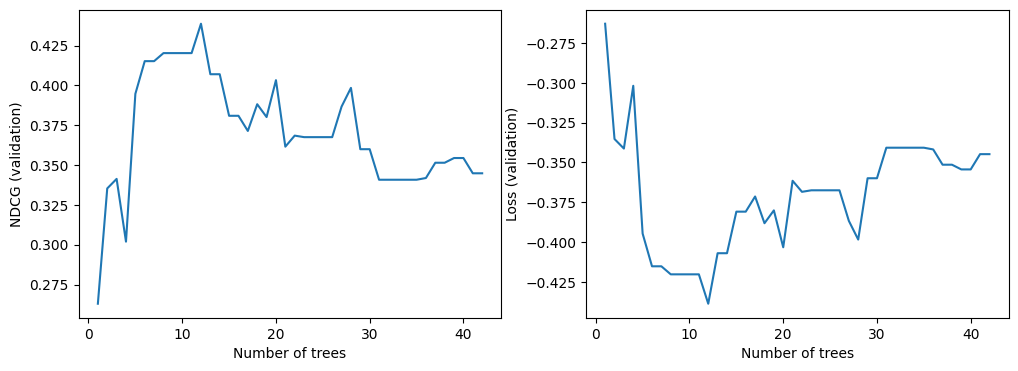
We can now look at the quality of the model on the validation dataset. By default, TF-DF trains ranking models to optimize the NDCG. The NDCG is a value between 0 and 1, where 1 is the perfect score. For this reason, -NDCG is the model loss.
import matplotlib.pyplot as plt

logs = model.make_inspector().training_logs()

plt.figure(figsize=(12, 4))

plt.subplot(1, 2, 1)
plt.plot([log.num_trees for log in logs], [log.evaluation.ndcg for log in logs])
plt.xlabel("Number of trees")
plt.ylabel("NDCG (validation)")

plt.subplot(1, 2, 2)
plt.plot([log.num_trees for log in logs], [log.evaluation.loss for log in logs])
plt.xlabel("Number of trees")
plt.ylabel("Loss (validation)")

plt.show()
As for all TF-DF models, you can also look at the model report (Note: The model report also contains the training logs):
%set_cell_height 400
model.summary()
<IPython.core.display.Javascript object>
Model: "gradient_boosted_trees_model"
_________________________________________________________________
 Layer (type)                Output Shape              Param #
=================================================================
=================================================================
Total params: 1 (1.00 Byte)
Trainable params: 0 (0.00 Byte)
Non-trainable params: 1 (1.00 Byte)
_________________________________________________________________
Type: "GRADIENT_BOOSTED_TREES"
Task: RANKING
Label: "__LABEL"
Rank group: "group"

Input Features (25):
    f_1
    f_10
    f_11
    f_12
    f_13
    f_14
    f_15
    f_16
    f_17
    f_18
    f_19
    f_2
    f_20
    f_21
    f_22
    f_23
    f_24
    f_25
    f_3
    f_4
    f_5
    f_6
    f_7
    f_8
    f_9

No weights

Variable Importance: INV_MEAN_MIN_DEPTH:

    1.  "f_9"  0.326164 ################
    2.  "f_3"  0.318071 ###############
    3.  "f_8"  0.308922 #############
    4.  "f_4"  0.271175 #########
    5. "f_19"  0.221570 ###
    6. "f_10"  0.215666 ##
    7. "f_11"  0.206509 #
    8. "f_22"  0.204742 #
    9. "f_25"  0.204497 #
   10. "f_23"  0.203238
   11. "f_21"  0.200830
   12. "f_24"  0.200445
   13. "f_12"  0.198840
   14. "f_18"  0.197676
   15. "f_20"  0.196634
   16.  "f_6"  0.196085
   17. "f_16"  0.196061
   18.  "f_2"  0.195683
   19.  "f_5"  0.195683
   20. "f_13"  0.195559
   21. "f_17"  0.195559

Variable Importance: NUM_AS_ROOT:

    1. "f_3"  4.000000 ################
    2. "f_4"  4.000000 ################
    3. "f_8"  3.000000 ##########
    4. "f_9"  1.000000

Variable Importance: NUM_NODES:

    1.  "f_8" 25.000000 ################
    2. "f_19" 18.000000 ###########
    3. "f_10" 15.000000 #########
    4.  "f_9" 14.000000 ########
    5.  "f_3" 13.000000 ########
    6. "f_23"  7.000000 ####
    7. "f_24"  6.000000 ###
    8. "f_11"  5.000000 ##
    9. "f_21"  5.000000 ##
   10. "f_25"  5.000000 ##
   11.  "f_4"  5.000000 ##
   12. "f_22"  4.000000 ##
   13. "f_12"  3.000000 #
   14. "f_20"  3.000000 #
   15. "f_16"  2.000000
   16.  "f_6"  2.000000
   17. "f_13"  1.000000
   18. "f_17"  1.000000
   19. "f_18"  1.000000
   20.  "f_2"  1.000000
   21.  "f_5"  1.000000

Variable Importance: SUM_SCORE:

    1.  "f_8" 10779.340861 ################
    2.  "f_9" 8831.772410 #############
    3.  "f_3" 4526.101184 ######
    4.  "f_4" 4360.245403 ######
    5. "f_19" 2325.288894 ###
    6. "f_10" 1881.848369 ##
    7. "f_21" 1674.980191 ##
    8. "f_11" 1127.632256 #
    9. "f_23" 1021.834252 #
   10. "f_24" 914.851512 #
   11. "f_22" 885.619576 #
   12. "f_25" 748.665007 #
   13. "f_20" 310.610858
   14. "f_16" 298.972842
   15.  "f_6" 212.376573
   16. "f_12" 130.725240
   17.  "f_2" 112.124991
   18. "f_18" 86.341193
   19.  "f_5" 65.103908
   20. "f_13" 57.966947
   21. "f_17" 21.930388


Loss: LAMBDA_MART_NDCG@5
Validation loss value: -0.438692
Number of trees per iteration: 1
Node format: NOT_SET
Number of trees: 12
Total number of nodes: 286

Number of nodes by tree:
Count: 12 Average: 23.8333 StdDev: 3.50793
Min: 17 Max: 29 Ignored: 0
----------------------------------------------
[ 17, 18) 1   8.33%   8.33% ###
[ 18, 19) 0   0.00%   8.33%
[ 19, 20) 1   8.33%  16.67% ###
[ 20, 21) 0   0.00%  16.67%
[ 21, 22) 2  16.67%  33.33% #######
[ 22, 23) 0   0.00%  33.33%
[ 23, 24) 1   8.33%  41.67% ###
[ 24, 25) 0   0.00%  41.67%
[ 25, 26) 3  25.00%  66.67% ##########
[ 26, 27) 0   0.00%  66.67%
[ 27, 28) 3  25.00%  91.67% ##########
[ 28, 29) 0   0.00%  91.67%
[ 29, 29] 1   8.33% 100.00% ###

Depth by leafs:
Count: 149 Average: 4.14094 StdDev: 1.08696
Min: 1 Max: 5 Ignored: 0
----------------------------------------------
[ 1, 2)  2   1.34%   1.34%
[ 2, 3) 18  12.08%  13.42% ##
[ 3, 4) 13   8.72%  22.15% ##
[ 4, 5) 40  26.85%  48.99% #####
[ 5, 5] 76  51.01% 100.00% ##########

Number of training obs by leaf:
Count: 149 Average: 673.691 StdDev: 2015.44
Min: 5 Max: 8211 Ignored: 0
----------------------------------------------
[    5,  415) 127  85.23%  85.23% ##########
[  415,  825)   6   4.03%  89.26%
[  825, 1236)   2   1.34%  90.60%
[ 1236, 1646)   0   0.00%  90.60%
[ 1646, 2056)   0   0.00%  90.60%
[ 2056, 2467)   1   0.67%  91.28%
[ 2467, 2877)   0   0.00%  91.28%
[ 2877, 3287)   0   0.00%  91.28%
[ 3287, 3698)   1   0.67%  91.95%
[ 3698, 4108)   0   0.00%  91.95%
[ 4108, 4518)   0   0.00%  91.95%
[ 4518, 4929)   1   0.67%  92.62%
[ 4929, 5339)   0   0.00%  92.62%
[ 5339, 5749)   0   0.00%  92.62%
[ 5749, 6160)   1   0.67%  93.29%
[ 6160, 6570)   0   0.00%  93.29%
[ 6570, 6980)   0   0.00%  93.29%
[ 6980, 7391)   0   0.00%  93.29%
[ 7391, 7801)   8   5.37%  98.66% #
[ 7801, 8211]   2   1.34% 100.00%

Attribute in nodes:
    25 : f_8 [NUMERICAL]
    18 : f_19 [NUMERICAL]
    15 : f_10 [NUMERICAL]
    14 : f_9 [NUMERICAL]
    13 : f_3 [NUMERICAL]
    7 : f_23 [NUMERICAL]
    6 : f_24 [NUMERICAL]
    5 : f_4 [NUMERICAL]
    5 : f_25 [NUMERICAL]
    5 : f_21 [NUMERICAL]
    5 : f_11 [NUMERICAL]
    4 : f_22 [NUMERICAL]
    3 : f_20 [NUMERICAL]
    3 : f_12 [NUMERICAL]
    2 : f_6 [NUMERICAL]
    2 : f_16 [NUMERICAL]
    1 : f_5 [NUMERICAL]
    1 : f_2 [NUMERICAL]
    1 : f_18 [NUMERICAL]
    1 : f_17 [NUMERICAL]
    1 : f_13 [NUMERICAL]

Attribute in nodes with depth <= 0:
    4 : f_4 [NUMERICAL]
    4 : f_3 [NUMERICAL]
    3 : f_8 [NUMERICAL]
    1 : f_9 [NUMERICAL]

Attribute in nodes with depth <= 1:
    11 : f_9 [NUMERICAL]
    9 : f_8 [NUMERICAL]
    4 : f_4 [NUMERICAL]
    4 : f_3 [NUMERICAL]
    1 : f_25 [NUMERICAL]
    1 : f_24 [NUMERICAL]
    1 : f_23 [NUMERICAL]
    1 : f_22 [NUMERICAL]
    1 : f_19 [NUMERICAL]
    1 : f_11 [NUMERICAL]

Attribute in nodes with depth <= 2:
    15 : f_8 [NUMERICAL]
    12 : f_9 [NUMERICAL]
    11 : f_3 [NUMERICAL]
    6 : f_19 [NUMERICAL]
    5 : f_4 [NUMERICAL]
    2 : f_25 [NUMERICAL]
    2 : f_11 [NUMERICAL]
    2 : f_10 [NUMERICAL]
    1 : f_24 [NUMERICAL]
    1 : f_23 [NUMERICAL]
    1 : f_22 [NUMERICAL]
    1 : f_18 [NUMERICAL]
    1 : f_17 [NUMERICAL]

Attribute in nodes with depth <= 3:
    22 : f_8 [NUMERICAL]
    13 : f_9 [NUMERICAL]
    11 : f_3 [NUMERICAL]
    10 : f_19 [NUMERICAL]
    9 : f_10 [NUMERICAL]
    5 : f_4 [NUMERICAL]
    5 : f_23 [NUMERICAL]
    5 : f_11 [NUMERICAL]
    4 : f_25 [NUMERICAL]
    4 : f_22 [NUMERICAL]
    4 : f_21 [NUMERICAL]
    3 : f_24 [NUMERICAL]
    2 : f_12 [NUMERICAL]
    1 : f_18 [NUMERICAL]
    1 : f_17 [NUMERICAL]

Attribute in nodes with depth <= 5:
    25 : f_8 [NUMERICAL]
    18 : f_19 [NUMERICAL]
    15 : f_10 [NUMERICAL]
    14 : f_9 [NUMERICAL]
    13 : f_3 [NUMERICAL]
    7 : f_23 [NUMERICAL]
    6 : f_24 [NUMERICAL]
    5 : f_4 [NUMERICAL]
    5 : f_25 [NUMERICAL]
    5 : f_21 [NUMERICAL]
    5 : f_11 [NUMERICAL]
    4 : f_22 [NUMERICAL]
    3 : f_20 [NUMERICAL]
    3 : f_12 [NUMERICAL]
    2 : f_6 [NUMERICAL]
    2 : f_16 [NUMERICAL]
    1 : f_5 [NUMERICAL]
    1 : f_2 [NUMERICAL]
    1 : f_18 [NUMERICAL]
    1 : f_17 [NUMERICAL]
    1 : f_13 [NUMERICAL]

Condition type in nodes:
    137 : HigherCondition
Condition type in nodes with depth <= 0:
    12 : HigherCondition
Condition type in nodes with depth <= 1:
    34 : HigherCondition
Condition type in nodes with depth <= 2:
    60 : HigherCondition
Condition type in nodes with depth <= 3:
    99 : HigherCondition
Condition type in nodes with depth <= 5:
    137 : HigherCondition

Training logs:
Number of iteration to final model: 12
    Iter:1 train-loss:-0.346669 valid-loss:-0.262935  train-NDCG@5:0.346669 valid-NDCG@5:0.262935
    Iter:2 train-loss:-0.412635 valid-loss:-0.335301  train-NDCG@5:0.412635 valid-NDCG@5:0.335301
    Iter:3 train-loss:-0.468270 valid-loss:-0.341295  train-NDCG@5:0.468270 valid-NDCG@5:0.341295
    Iter:4 train-loss:-0.481511 valid-loss:-0.301897  train-NDCG@5:0.481511 valid-NDCG@5:0.301897
    Iter:5 train-loss:-0.473165 valid-loss:-0.394670  train-NDCG@5:0.473165 valid-NDCG@5:0.394670
    Iter:6 train-loss:-0.496260 valid-loss:-0.415201  train-NDCG@5:0.496260 valid-NDCG@5:0.415201
    Iter:16 train-loss:-0.526791 valid-loss:-0.380900  train-NDCG@5:0.526791 valid-NDCG@5:0.380900
    Iter:26 train-loss:-0.560398 valid-loss:-0.367496  train-NDCG@5:0.560398 valid-NDCG@5:0.367496
    Iter:36 train-loss:-0.584252 valid-loss:-0.341845  train-NDCG@5:0.584252 valid-NDCG@5:0.341845
And if you are curious, you can also plot the model:
tfdf.model_plotter.plot_model_in_colab(model, tree_idx=0, max_depth=3)
Predicting with a ranking model
For an incoming query, we can use our ranking model to predict the relevance of a stack of documents. In practice this means that for each query, we must come up with a set of documents that may or may not be relevant to the query. We call these documents our candidate documents. For each pair query/candidate document, we can compute the same features used during training. This is our serving dataset.
Going back to the example from the beginning of this tutorial, the serving dataset might look like this:
| query | document_id | feature_1 | feature_2 |
|---|---|---|---|
| fish | 32 | 0.3 | blue |
| fish | 33 | 1.0 | green |
| fish | 34 | 0.4 | blue |
| fish | 35 | NA | brown |
Observe that relevance is not part of the serving dataset, since this is what the model is trying to predict.
The serving dataset is fed to the TF-DF model and assigns a relevance score to each document.
| query | document_id | feature_1 | feature_2 | relevance |
|---|---|---|---|---|
| fish | 32 | 0.3 | blue | 0.325 |
| fish | 33 | 1.0 | green | 0.125 |
| fish | 34 | 0.4 | blue | 0.155 |
| fish | 35 | NA | brown | 0.593 |
This means that the document with document_id 35 is predicted to be most relevant for query "fish".
Let's try to do this with our real model.
# Path to a test dataset using libsvm format.
test_dataset_path = os.path.join(os.path.dirname(archive_path),"OHSUMED/Data/Fold1/testset.txt")
# Convert the dataset.
csv_test_dataset_path="/tmp/ohsumed_test.csv"
convert_libsvm_to_csv(raw_dataset_path, csv_test_dataset_path)

# Load a dataset into a Pandas Dataframe.
test_dataset_df = pd.read_csv(csv_test_dataset_path)

# Display the first 3 examples.
test_dataset_df.head(3)
Suppose our query is "g_5" and the test dataset already contains the candidate documents for this query.
# Filter by "g_5"
serving_dataset_df = test_dataset_df[test_dataset_df['group'] == 'g_5']
# Remove the columns for group and relevance, not needed for predictions.
serving_dataset_df = serving_dataset_df.drop(['relevance', 'group'], axis=1)
# Convert to a Tensorflow dataset
serving_dataset_ds = tfdf.keras.pd_dataframe_to_tf_dataset(serving_dataset_df, task=tfdf.keras.Task.RANKING)
# Run predictions with on all candidate documents
predictions = model.predict(serving_dataset_ds)
1/1 [==============================] - 0s 140ms/step
We can use add the predictions to the dataframe and use them to find the documents with the highest scores.
serving_dataset_df['prediction_score'] = predictions
serving_dataset_df.sort_values(by=['prediction_score'], ascending=False).head()