Neural Structured Learning 프레임워크
컬렉션을 사용해 정리하기
내 환경설정을 기준으로 콘텐츠를 저장하고 분류하세요.
Neural Structured Learning(NSL)은 특성 입력과 함께 구조적 신호(사용 가능한 경우)를 활용하여 심층 신경망 훈련에 중점을 둡니다. Bui et al. (WSDM'18)에서 소개된 구조적 신호는 신경망의 훈련을 정규화하는 데 사용되며, 모델이 정확한 예측값(감독 손실을 최소화함으로써)을 학습하도록 하는 동시에 입력의 구조적 유사성을 유지합니다(이웃 손실 최소화, 아래 그림 참조). 이 기술은 일반적이며 임의의 신경 아키텍처(예: Feed-forward NN, Convolutional NN 및 Recurrent NN)에 적용될 수 있습니다.

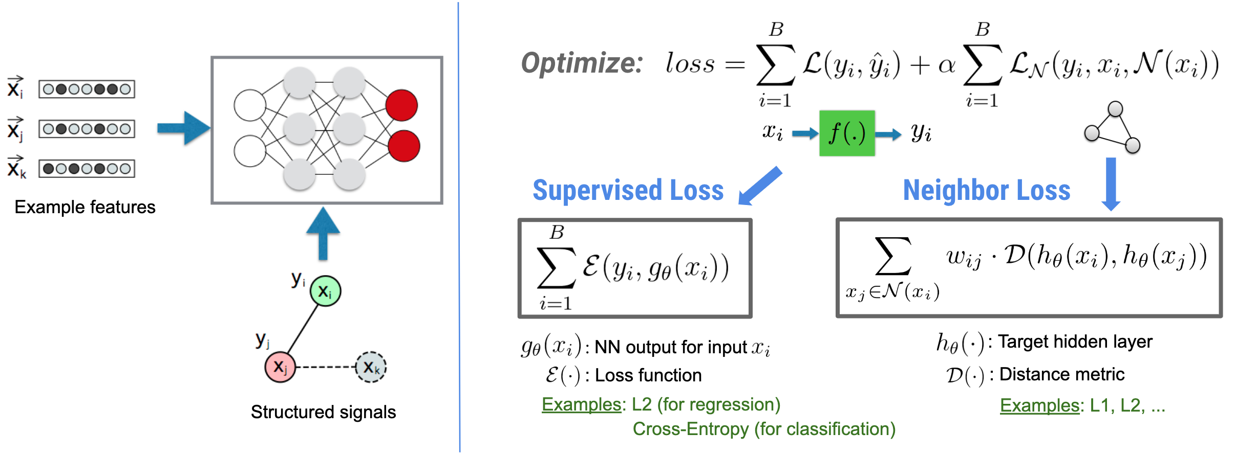
일반화된 이웃 손실 수식은 유연하며 위에 설명된 것과 다른 형태를 가질 수 있습니다. 예를 들어, \(\sum_{x_j \in \mathcal{N}(x_i)}\mathcal{E}(y_i,g_\theta(x_j))\)를 이웃 손실로 선택할 수도 있으며, 실제 \(y_i\)과 이웃 \(g_\theta(x_j)\)의 예측 사이의 거리를 계산합니다. 일반적으로 적대적 학습(Goodfellow et al., ICLR'15)에 사용됩니다. 따라서 이웃이 그래프로 명시적으로 표현되는 경우, NSL은 신경 그래프 학습으로 일반화되고, 이웃이 적대적 교란(perturbation)에 의해 암시적으로 유도되는 경우, 적대적 학습으로 일반화됩니다.
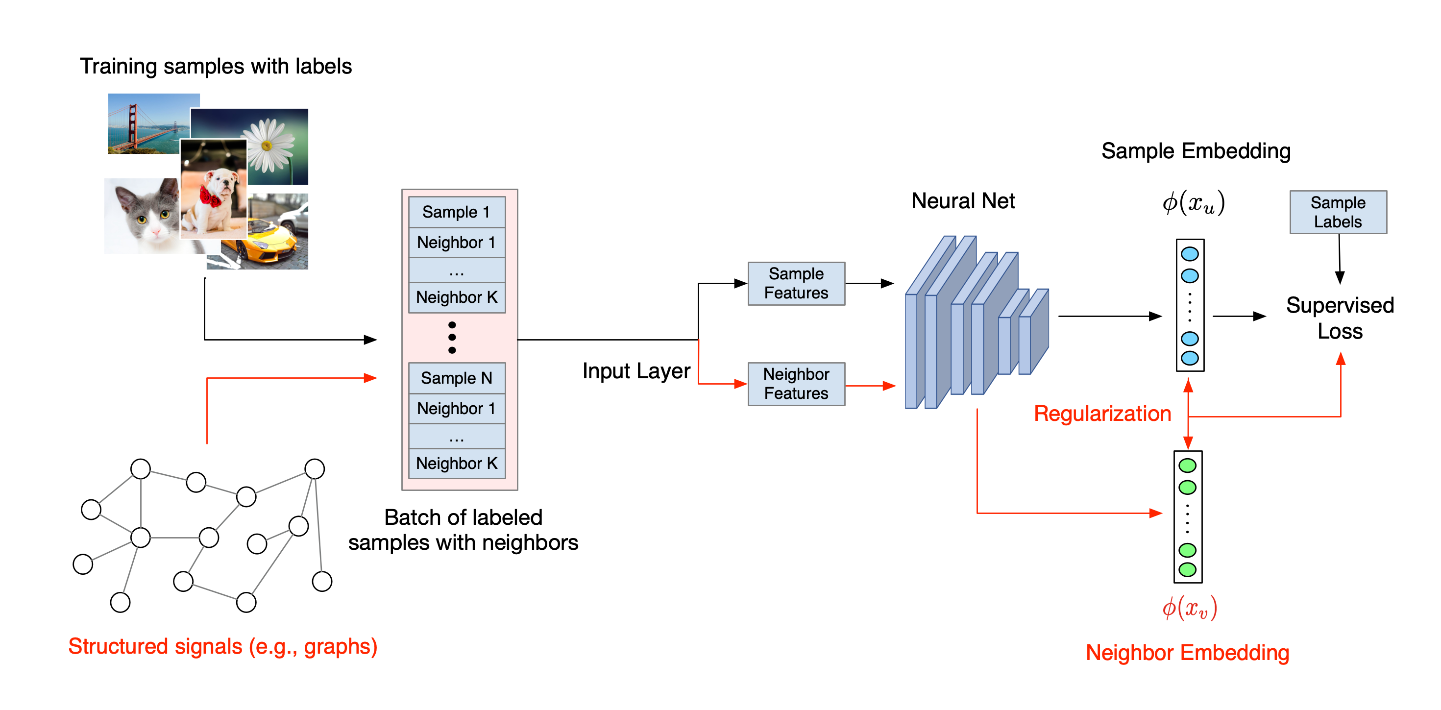
Neural Structured Learning의 전체 워크플로는 다음과 같습니다. 검은색 화살표는 기존 훈련 워크플로를 나타내고, 빨간색 화살표는 구조적 신호를 활용하기 위해 NSL에서 도입한 새로운 워크플로를 나타냅니다. 첫째, 훈련 샘플은 구조적 신호를 포함하도록 확대됩니다. 구조적 신호가 명시적으로 제공되지 않으면 구성되거나 유도될 수 있습니다(후자는 적대적 학습에 적용됨). 다음으로, 증강 훈련 샘플(원래 샘플과 해당 이웃 모두 포함)은 임베딩을 계산하기 위해 신경망에 공급됩니다. 샘플의 임베딩과 이웃 임베딩 사이의 거리가 계산되어 이웃 손실로 사용되며, 이는 정규화 항으로 처리되고 최종 손실에 추가됩니다. 명시적인 이웃 기반 정규화의 경우, 일반적으로 이웃 손실을 샘플의 임베딩과 이웃 임베딩 사이의 거리로 계산합니다. 그러나 신경망의 모든 레이어가 이웃 손실을 계산하는 데 사용될 수 있습니다. 반면에 유도된 이웃 기반 정규화(적대적)의 경우, 유도된 적대적 이웃의 출력 예측과 실제 레이블 사이의 거리로 이웃 손실을 계산합니다.

왜 NSL을 사용하나요?
NSL은 다음과 같은 이점을 제공합니다.
단계별 튜토리얼
Neural Structured Learning에 대한 실습 경험을 얻기 위해 구조적 신호를 명시적으로 제공, 유도 또는 구성할 수 있는 다양한 시나리오를 다루는 3가지 튜토리얼이 제공됩니다.
달리 명시되지 않는 한 이 페이지의 콘텐츠에는 Creative Commons Attribution 4.0 라이선스에 따라 라이선스가 부여되며, 코드 샘플에는 Apache 2.0 라이선스에 따라 라이선스가 부여됩니다. 자세한 내용은 Google Developers 사이트 정책을 참조하세요. 자바는 Oracle 및/또는 Oracle 계열사의 등록 상표입니다.
최종 업데이트: 2024-02-12(UTC)
[null,null,["최종 업데이트: 2024-02-12(UTC)"],[],[],null,["# The Neural Structured Learning Framework\n\nNeural Structured Learning (NSL) focuses on training deep neural networks by\nleveraging structured signals (when available) along with feature inputs. As\nintroduced by [Bui et al. (WSDM'18)](https://research.google/pubs/pub46568.pdf),\nthese structured signals are used to regularize the training of a neural\nnetwork, forcing the model to learn accurate predictions (by minimizing\nsupervised loss), while at the same time maintaining the input structural\nsimilarity (by minimizing the neighbor loss, see the figure below). This\ntechnique is generic and can be applied on arbitrary neural architectures (such\nas Feed-forward NNs, Convolutional NNs and Recurrent NNs).\n\nNote that the generalized neighbor loss equation is flexible and can have other\nforms besides the one illustrated above. For example, we can also select\n\\\\(\\\\sum_{x_j \\\\in \\\\mathcal{N}(x_i)}\\\\mathcal{E}(y_i,g_\\\\theta(x_j))\\\\) to be the\nneighbor loss, which calculates the distance between the ground truth \\\\(y_i\\\\)\nand the prediction from the neighbor \\\\(g_\\\\theta(x_j)\\\\). This is commonly used in\nadversarial learning\n[(Goodfellow et al., ICLR'15)](https://arxiv.org/pdf/1412.6572.pdf). Therefore,\nNSL generalizes to **Neural Graph Learning** if neighbors are explicitly\nrepresented by a graph, and to **Adversarial Learning** if neighbors are\nimplicitly induced by adversarial perturbation.\n\nThe overall workflow for Neural Structured Learning is illustrated below. Black\narrows represent the conventional training workflow and red arrows represent the\nnew workflow as introduced by NSL to leverage structured signals. First, the\ntraining samples are augmented to include structured signals. When structured\nsignals are not explicitly provided, they can be either constructed or induced\n(the latter applies to adversarial learning). Next, the augmented training\nsamples (including both original samples and their corresponding neighbors) are\nfed to the neural network for calculating their embeddings. The distance between\na sample's embedding and its neighbor's embedding is calculated and used as the\nneighbor loss, which is treated as a regularization term and added to the final\nloss. For explicit neighbor-based regularization, we typically compute the\nneighbor loss as the distance between the sample's embedding and the neighbor's\nembedding. However, any layer of the neural network may be used to compute the\nneighbor loss. On the other hand, for induced neighbor-based regularization\n(adversarial), we compute the neighbor loss as the distance between the output\nprediction of the induced adversarial neighbor and the ground truth label.\n\nWhy use NSL?\n------------\n\nNSL brings the following advantages:\n\n- **Higher accuracy** : the structured signal(s) among samples can provide information that is not always available in feature inputs; therefore, the joint training approach (with both structured signals and features) has been shown to outperform many existing methods (that rely on training with features only) on a wide range of tasks, such as document classification and semantic intent classification ([Bui et al., WSDM'18](https://research.google/pubs/pub46568.pdf) \\& [Kipf et al., ICLR'17](https://arxiv.org/pdf/1609.02907.pdf)).\n- **Robustness** : models trained with adversarial examples have been shown to be robust against adversarial perturbations designed for misleading a model's prediction or classification ([Goodfellow et al., ICLR'15](https://arxiv.org/pdf/1412.6572.pdf) \\& [Miyato et al., ICLR'16](https://arxiv.org/pdf/1704.03976.pdf)). When the number of training samples is small, training with adversarial examples also helps improve model accuracy ([Tsipras et al., ICLR'19](https://arxiv.org/pdf/1805.12152.pdf)).\n- **Less labeled data required** : NSL enables neural networks to harness both labeled and unlabeled data, which extends the learning paradigm to [semi-supervised learning](https://en.wikipedia.org/wiki/Semi-supervised_learning). Specifically, NSL allows the network to train using labeled data as in the supervised setting, and at the same time drives the network to learn similar hidden representations for the \"neighboring samples\" that may or may not have labels. This technique has shown great promise for improving model accuracy when the amount of labeled data is relatively small ([Bui et al., WSDM'18](https://research.google/pubs/pub46568.pdf) \\& [Miyato et al., ICLR'16](https://arxiv.org/pdf/1704.03976.pdf)).\n\nStep-by-step Tutorials\n----------------------\n\nTo obtain hands-on experience with Neural Structured Learning, we have tutorials\nthat cover various scenarios where structured signals may be explicitly given,\nconstructed, or induced. Here are a few:\n\n- [Graph regularization for document classification using natural graphs](/neural_structured_learning/tutorials/graph_keras_mlp_cora).\n In this tutorial, we explore the use of graph regularization to classify\n documents that form a natural (organic) graph.\n\n- [Graph regularization for sentiment classification using synthesized graphs](/neural_structured_learning/tutorials/graph_keras_lstm_imdb).\n In this tutorial, we demonstrate the use of graph regularization to classify\n movie review sentiments by constructing (synthesizing) structured signals.\n\n- [Adversarial learning for image classification](/neural_structured_learning/tutorials/adversarial_keras_cnn_mnist).\n In this tutorial, we explore the use of adversarial learning (where\n structured signals are induced) to classify images containing numeric\n digits.\n\nMore examples and tutorials can be found in the\n[examples](https://github.com/tensorflow/neural-structured-learning/tree/master/neural_structured_learning/examples)\ndirectory of our GitHub repository."]]