ニューラル構造化学習フレームワーク
コレクションでコンテンツを整理
必要に応じて、コンテンツの保存と分類を行います。
ニューラル構造化学習(NSL)は、構造化シグナル(利用可能な場合)を特徴入力と共に活用してディープニューラルネットワークをトレーニングすることに焦点を当てています。Bui et al.(WSDM'18)が紹介しているように、これらの構造化された信号をニューラルネットワークのトレーニングを正則化するために使用し、(教師あり損失を最小化することで)モデルに正確な予測値を学習させると同時に、(近傍損失を最小化することで)入力の構造的類似性を維持します(下の図をご覧ください)。これは一般的な手法であり、任意のニューラルアーキテクチャ(フィードフォワード NN、畳み込み NN、再帰型 NN など)に適用することができます。

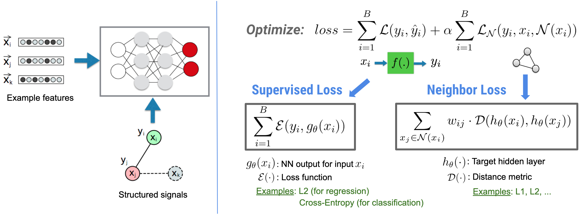
一般化された近傍損失の方程式には柔軟性があり、上で示した以外の形をとることができるので、注意が必要です。例えば、近傍損失に \(\sum_{x_j \in \mathcal{N}(x_i)}\mathcal{E}(y_i,g_\theta(x_j))\) を選択して、真の正解 \($y_i\) と近傍 \(\)g_\theta(x_j)\(\) からの予測値との間の距離を計算することも可能です。これは敵対的学習でよく使用されています(Goodfellow et al., ICLR'15)。つまり NSL は、近傍が明示的にグラフで表現されている場合はニューラルグラフ学習に、近傍が暗黙的に敵対的摂動で誘導されている場合は敵対的学習に一般化します。
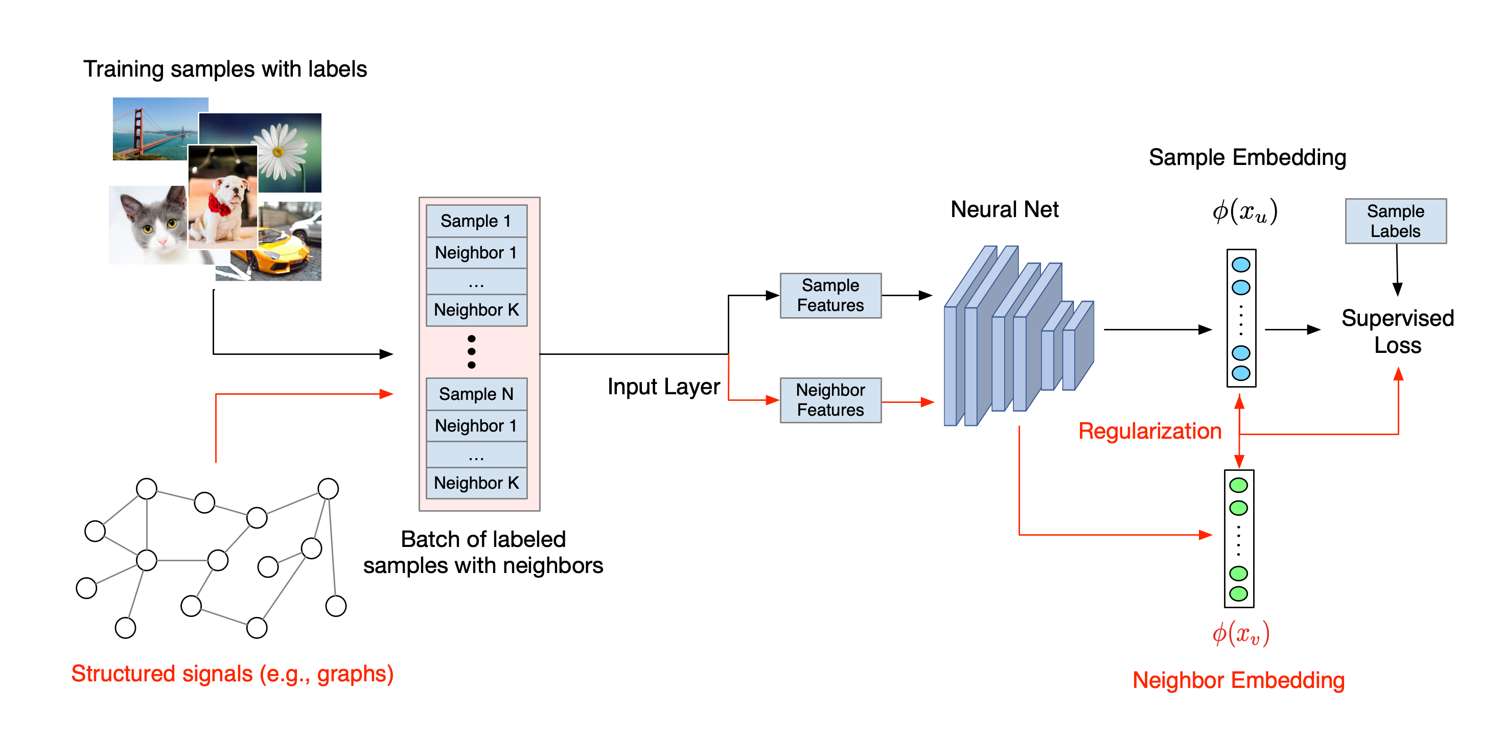
ニューラル構造化学習の全体的なワークフローを以下に示します。黒い矢印は従来のトレーニングワークフロー、赤い矢印は構造化された信号を活用するために NSL が導入した新しいワークフローを示しています。まず、トレーニングサンプルを増強して構造化された信号が含まれるようにします。構造化された信号が明示的に提供されない場合は、信号が構築されているか誘導されている可能性があります(誘導された信号は敵対的学習に適用されます)。次に、増強されたトレーニングサンプル(元のサンプルとそれに対応する近傍サンプルの両方を含む)をニューラルネットワークに供給して、それらの埋め込みを計算します。サンプル埋め込みと近傍埋め込みの間の距離を計算して近傍損失として使用し、これが正則化項とみなされて最終的な損失に加算されます。通常、近傍ベースの明示的な正則化には、サンプル埋め込みと近傍埋め込み間の距離で近傍損失を計算します。ただし、近傍損失の計算にはニューラルネットワークのどのレイヤーでも使用できます。一方、誘導された近傍ベースの正則化(敵対的)には、誘導された敵対的近傍の出力予測と真の正解ラベルとの間の距離で近傍損失を計算します。

NSL を選ぶ理由
NSL には以下のようなメリットがあります。
段階的なチュートリアル
ニューラル構造化学習の実戦経験を得られるよう、構造化シグナルが明示的に指定される場合、構築される場合、または誘導される場合など、さまざまなシナリオをカバーするチュートリアルを用意しています。以下にその一部を紹介します。
その他の例やチュートリアルは、GitHub リポジトリの examples ディレクトリをご覧ください。
特に記載のない限り、このページのコンテンツはクリエイティブ・コモンズの表示 4.0 ライセンスにより使用許諾されます。コードサンプルは Apache 2.0 ライセンスにより使用許諾されます。詳しくは、Google Developers サイトのポリシーをご覧ください。Java は Oracle および関連会社の登録商標です。
最終更新日 2022-08-09 UTC。
[null,null,["最終更新日 2022-08-09 UTC。"],[],[],null,["# The Neural Structured Learning Framework\n\nNeural Structured Learning (NSL) focuses on training deep neural networks by\nleveraging structured signals (when available) along with feature inputs. As\nintroduced by [Bui et al. (WSDM'18)](https://research.google/pubs/pub46568.pdf),\nthese structured signals are used to regularize the training of a neural\nnetwork, forcing the model to learn accurate predictions (by minimizing\nsupervised loss), while at the same time maintaining the input structural\nsimilarity (by minimizing the neighbor loss, see the figure below). This\ntechnique is generic and can be applied on arbitrary neural architectures (such\nas Feed-forward NNs, Convolutional NNs and Recurrent NNs).\n\nNote that the generalized neighbor loss equation is flexible and can have other\nforms besides the one illustrated above. For example, we can also select\n\\\\(\\\\sum_{x_j \\\\in \\\\mathcal{N}(x_i)}\\\\mathcal{E}(y_i,g_\\\\theta(x_j))\\\\) to be the\nneighbor loss, which calculates the distance between the ground truth \\\\(y_i\\\\)\nand the prediction from the neighbor \\\\(g_\\\\theta(x_j)\\\\). This is commonly used in\nadversarial learning\n[(Goodfellow et al., ICLR'15)](https://arxiv.org/pdf/1412.6572.pdf). Therefore,\nNSL generalizes to **Neural Graph Learning** if neighbors are explicitly\nrepresented by a graph, and to **Adversarial Learning** if neighbors are\nimplicitly induced by adversarial perturbation.\n\nThe overall workflow for Neural Structured Learning is illustrated below. Black\narrows represent the conventional training workflow and red arrows represent the\nnew workflow as introduced by NSL to leverage structured signals. First, the\ntraining samples are augmented to include structured signals. When structured\nsignals are not explicitly provided, they can be either constructed or induced\n(the latter applies to adversarial learning). Next, the augmented training\nsamples (including both original samples and their corresponding neighbors) are\nfed to the neural network for calculating their embeddings. The distance between\na sample's embedding and its neighbor's embedding is calculated and used as the\nneighbor loss, which is treated as a regularization term and added to the final\nloss. For explicit neighbor-based regularization, we typically compute the\nneighbor loss as the distance between the sample's embedding and the neighbor's\nembedding. However, any layer of the neural network may be used to compute the\nneighbor loss. On the other hand, for induced neighbor-based regularization\n(adversarial), we compute the neighbor loss as the distance between the output\nprediction of the induced adversarial neighbor and the ground truth label.\n\nWhy use NSL?\n------------\n\nNSL brings the following advantages:\n\n- **Higher accuracy** : the structured signal(s) among samples can provide information that is not always available in feature inputs; therefore, the joint training approach (with both structured signals and features) has been shown to outperform many existing methods (that rely on training with features only) on a wide range of tasks, such as document classification and semantic intent classification ([Bui et al., WSDM'18](https://research.google/pubs/pub46568.pdf) \\& [Kipf et al., ICLR'17](https://arxiv.org/pdf/1609.02907.pdf)).\n- **Robustness** : models trained with adversarial examples have been shown to be robust against adversarial perturbations designed for misleading a model's prediction or classification ([Goodfellow et al., ICLR'15](https://arxiv.org/pdf/1412.6572.pdf) \\& [Miyato et al., ICLR'16](https://arxiv.org/pdf/1704.03976.pdf)). When the number of training samples is small, training with adversarial examples also helps improve model accuracy ([Tsipras et al., ICLR'19](https://arxiv.org/pdf/1805.12152.pdf)).\n- **Less labeled data required** : NSL enables neural networks to harness both labeled and unlabeled data, which extends the learning paradigm to [semi-supervised learning](https://en.wikipedia.org/wiki/Semi-supervised_learning). Specifically, NSL allows the network to train using labeled data as in the supervised setting, and at the same time drives the network to learn similar hidden representations for the \"neighboring samples\" that may or may not have labels. This technique has shown great promise for improving model accuracy when the amount of labeled data is relatively small ([Bui et al., WSDM'18](https://research.google/pubs/pub46568.pdf) \\& [Miyato et al., ICLR'16](https://arxiv.org/pdf/1704.03976.pdf)).\n\nStep-by-step Tutorials\n----------------------\n\nTo obtain hands-on experience with Neural Structured Learning, we have tutorials\nthat cover various scenarios where structured signals may be explicitly given,\nconstructed, or induced. Here are a few:\n\n- [Graph regularization for document classification using natural graphs](/neural_structured_learning/tutorials/graph_keras_mlp_cora).\n In this tutorial, we explore the use of graph regularization to classify\n documents that form a natural (organic) graph.\n\n- [Graph regularization for sentiment classification using synthesized graphs](/neural_structured_learning/tutorials/graph_keras_lstm_imdb).\n In this tutorial, we demonstrate the use of graph regularization to classify\n movie review sentiments by constructing (synthesizing) structured signals.\n\n- [Adversarial learning for image classification](/neural_structured_learning/tutorials/adversarial_keras_cnn_mnist).\n In this tutorial, we explore the use of adversarial learning (where\n structured signals are induced) to classify images containing numeric\n digits.\n\nMore examples and tutorials can be found in the\n[examples](https://github.com/tensorflow/neural-structured-learning/tree/master/neural_structured_learning/examples)\ndirectory of our GitHub repository."]]