神经结构学习框架
使用集合让一切井井有条
根据您的偏好保存内容并对其进行分类。
神经结构学习 (NSL) 侧重于通过利用结构化信号(可用时)和特征输入来训练深度神经网络。如 Bui 等人在 WSDM'18 上提出的那样,这些结构化信号用于对神经网络训练执行正则化,迫使模型学习准确的预测(通过最小化监督损失),同时保持输入的结构相似度(通过最小化近邻损失,请参见下图)。此技术是适用于任意神经网络架构(例如前馈神经网络、卷积神经网络和循环神经网络)的通用型技术。

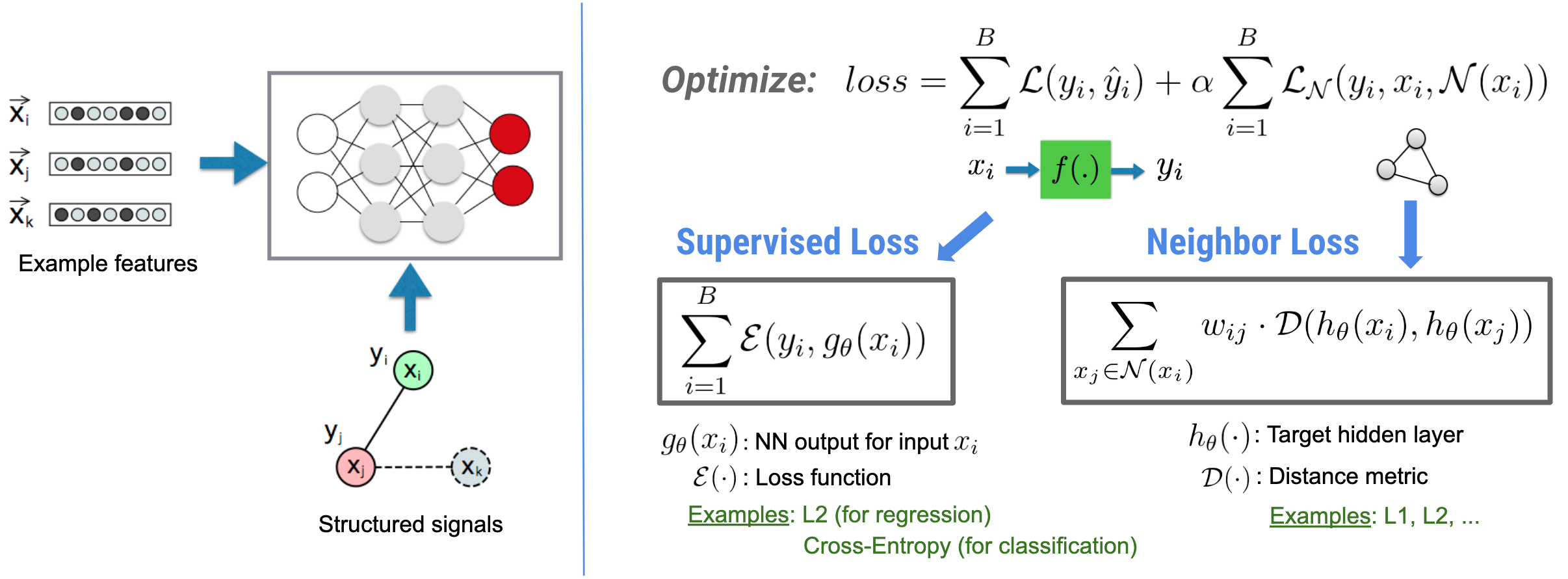
请注意,泛化的近邻损失方程非常灵活,可具有除上例所示以外的其他形式。例如,我们还可以选择 \(\sum_{x_j \in \mathcal{N}(x_i)}\mathcal{E}(y_i,g_\theta(x_j))\) 作为近邻损失,用于计算真实 \(y_i\) 与从近邻 \(g_\theta(x_j)\) 预测的值之间的距离。这是对抗学习(Goodfellow 等人在 ICLR'15 上提出)中的常用方法。因此,如果近邻通过计算图显式表示,则 NSL 可泛化到神经计算图学习;如果近邻由对抗扰动隐式诱导,则泛化到对抗学习。
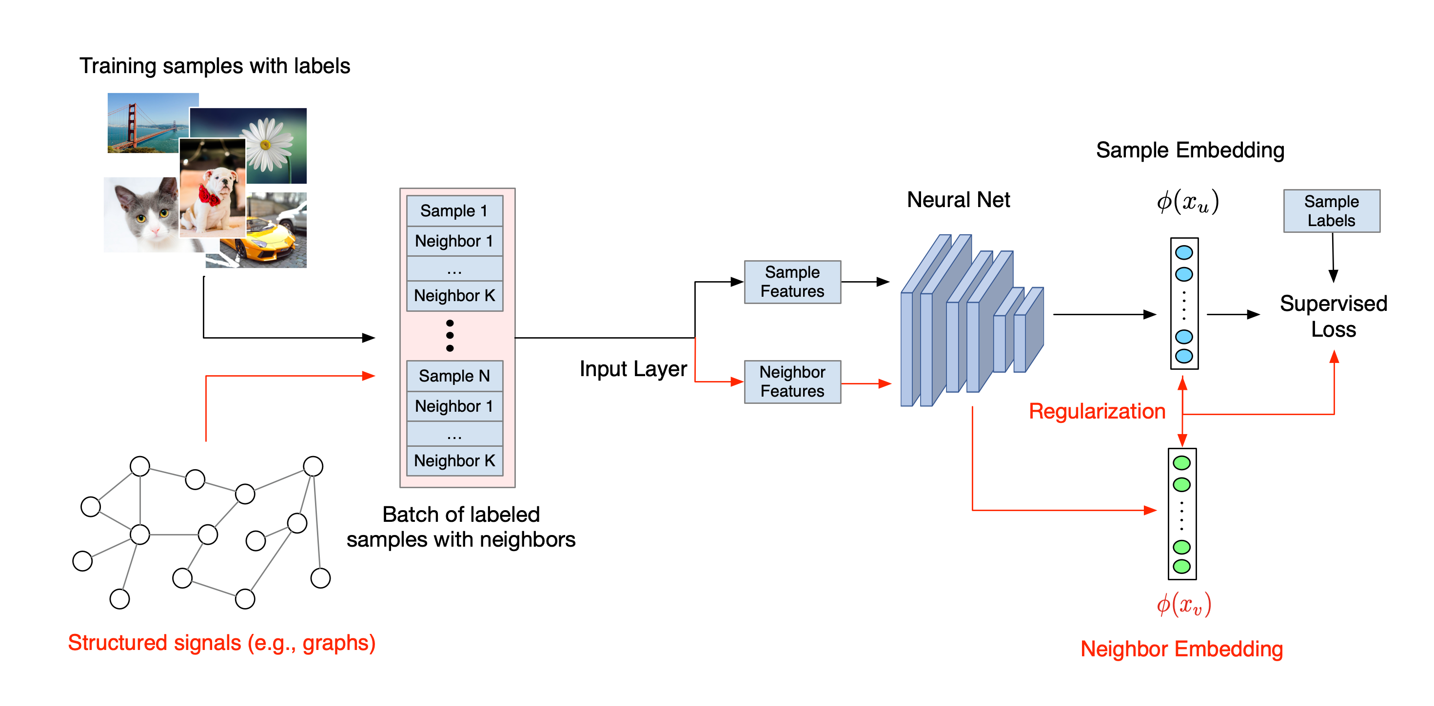
神经结构学习的整体工作流如下所示。黑色箭头代表常规训练工作流,红色箭头代表 NSL 为利用结构化信号而引入的新工作流。首先,对训练样本进行增强以包含结构化信号。如果没有显式提供结构化信号,则可以构造或诱导结构化信号(后者适用于对抗学习)。接下来,将增强的训练样本(包括原始样本及其相应近邻)馈送到神经网络以计算其嵌入向量。计算样本的嵌入向量与其近邻的嵌入向量之间的距离,并用作近邻损失,将其处理为正则化项并添加到最终损失中。对于基于显式近邻的正则化,我们通常将近邻损失计算为样本嵌入向量与近邻嵌入向量之间的距离。但是,神经网络的任一层都可以用来计算近邻损失。另一方面,对于基于诱导近邻的正则化(对抗),我们将近邻损失计算为诱导对抗近邻的输出预测与真实标签之间的距离。

为何使用 NSL?
NSL 可提供以下优势:
分步教程
为了帮助您获得神经结构学习的动手经验,我们提供了各种教程,涵盖显式给定、构造或诱导结构化信号等各种场景。下面是一些示例:
可以在我们 GitHub 仓库的示例目录中找到更多示例和教程。
如未另行说明,那么本页面中的内容已根据知识共享署名 4.0 许可获得了许可,并且代码示例已根据 Apache 2.0 许可获得了许可。有关详情,请参阅 Google 开发者网站政策。Java 是 Oracle 和/或其关联公司的注册商标。
最后更新时间 (UTC):2022-06-07。
[null,null,["最后更新时间 (UTC):2022-06-07。"],[],[],null,["# The Neural Structured Learning Framework\n\nNeural Structured Learning (NSL) focuses on training deep neural networks by\nleveraging structured signals (when available) along with feature inputs. As\nintroduced by [Bui et al. (WSDM'18)](https://research.google/pubs/pub46568.pdf),\nthese structured signals are used to regularize the training of a neural\nnetwork, forcing the model to learn accurate predictions (by minimizing\nsupervised loss), while at the same time maintaining the input structural\nsimilarity (by minimizing the neighbor loss, see the figure below). This\ntechnique is generic and can be applied on arbitrary neural architectures (such\nas Feed-forward NNs, Convolutional NNs and Recurrent NNs).\n\nNote that the generalized neighbor loss equation is flexible and can have other\nforms besides the one illustrated above. For example, we can also select\n\\\\(\\\\sum_{x_j \\\\in \\\\mathcal{N}(x_i)}\\\\mathcal{E}(y_i,g_\\\\theta(x_j))\\\\) to be the\nneighbor loss, which calculates the distance between the ground truth \\\\(y_i\\\\)\nand the prediction from the neighbor \\\\(g_\\\\theta(x_j)\\\\). This is commonly used in\nadversarial learning\n[(Goodfellow et al., ICLR'15)](https://arxiv.org/pdf/1412.6572.pdf). Therefore,\nNSL generalizes to **Neural Graph Learning** if neighbors are explicitly\nrepresented by a graph, and to **Adversarial Learning** if neighbors are\nimplicitly induced by adversarial perturbation.\n\nThe overall workflow for Neural Structured Learning is illustrated below. Black\narrows represent the conventional training workflow and red arrows represent the\nnew workflow as introduced by NSL to leverage structured signals. First, the\ntraining samples are augmented to include structured signals. When structured\nsignals are not explicitly provided, they can be either constructed or induced\n(the latter applies to adversarial learning). Next, the augmented training\nsamples (including both original samples and their corresponding neighbors) are\nfed to the neural network for calculating their embeddings. The distance between\na sample's embedding and its neighbor's embedding is calculated and used as the\nneighbor loss, which is treated as a regularization term and added to the final\nloss. For explicit neighbor-based regularization, we typically compute the\nneighbor loss as the distance between the sample's embedding and the neighbor's\nembedding. However, any layer of the neural network may be used to compute the\nneighbor loss. On the other hand, for induced neighbor-based regularization\n(adversarial), we compute the neighbor loss as the distance between the output\nprediction of the induced adversarial neighbor and the ground truth label.\n\nWhy use NSL?\n------------\n\nNSL brings the following advantages:\n\n- **Higher accuracy** : the structured signal(s) among samples can provide information that is not always available in feature inputs; therefore, the joint training approach (with both structured signals and features) has been shown to outperform many existing methods (that rely on training with features only) on a wide range of tasks, such as document classification and semantic intent classification ([Bui et al., WSDM'18](https://research.google/pubs/pub46568.pdf) \\& [Kipf et al., ICLR'17](https://arxiv.org/pdf/1609.02907.pdf)).\n- **Robustness** : models trained with adversarial examples have been shown to be robust against adversarial perturbations designed for misleading a model's prediction or classification ([Goodfellow et al., ICLR'15](https://arxiv.org/pdf/1412.6572.pdf) \\& [Miyato et al., ICLR'16](https://arxiv.org/pdf/1704.03976.pdf)). When the number of training samples is small, training with adversarial examples also helps improve model accuracy ([Tsipras et al., ICLR'19](https://arxiv.org/pdf/1805.12152.pdf)).\n- **Less labeled data required** : NSL enables neural networks to harness both labeled and unlabeled data, which extends the learning paradigm to [semi-supervised learning](https://en.wikipedia.org/wiki/Semi-supervised_learning). Specifically, NSL allows the network to train using labeled data as in the supervised setting, and at the same time drives the network to learn similar hidden representations for the \"neighboring samples\" that may or may not have labels. This technique has shown great promise for improving model accuracy when the amount of labeled data is relatively small ([Bui et al., WSDM'18](https://research.google/pubs/pub46568.pdf) \\& [Miyato et al., ICLR'16](https://arxiv.org/pdf/1704.03976.pdf)).\n\nStep-by-step Tutorials\n----------------------\n\nTo obtain hands-on experience with Neural Structured Learning, we have tutorials\nthat cover various scenarios where structured signals may be explicitly given,\nconstructed, or induced. Here are a few:\n\n- [Graph regularization for document classification using natural graphs](/neural_structured_learning/tutorials/graph_keras_mlp_cora).\n In this tutorial, we explore the use of graph regularization to classify\n documents that form a natural (organic) graph.\n\n- [Graph regularization for sentiment classification using synthesized graphs](/neural_structured_learning/tutorials/graph_keras_lstm_imdb).\n In this tutorial, we demonstrate the use of graph regularization to classify\n movie review sentiments by constructing (synthesizing) structured signals.\n\n- [Adversarial learning for image classification](/neural_structured_learning/tutorials/adversarial_keras_cnn_mnist).\n In this tutorial, we explore the use of adversarial learning (where\n structured signals are induced) to classify images containing numeric\n digits.\n\nMore examples and tutorials can be found in the\n[examples](https://github.com/tensorflow/neural-structured-learning/tree/master/neural_structured_learning/examples)\ndirectory of our GitHub repository."]]