Noise

Noise is present in modern day quantum computers. Qubits are susceptible to interference from the surrounding environment, imperfect fabrication, TLS and sometimes even gamma rays. Until large scale error correction is reached, the algorithms of today must be able to remain functional in the presence of noise. This makes testing algorithms under noise an important step for validating quantum algorithms / models will function on the quantum computers of today.

In this tutorial you will explore the basics of noisy circuit simulation in TFQ via the high level tfq.layers API.

Setup

pip install tensorflow==2.15.0 tensorflow-quantum==0.7.3

pip install -q git+https://github.com/tensorflow/docs

# Update package resources to account for version changes.
import importlib, pkg_resources
importlib.reload(pkg_resources)

/tmpfs/tmp/ipykernel_32316/1875984233.py:2: DeprecationWarning: pkg_resources is deprecated as an API. See https://setuptools.pypa.io/en/latest/pkg_resources.html
  import importlib, pkg_resources
<module 'pkg_resources' from '/tmpfs/src/tf_docs_env/lib/python3.9/site-packages/pkg_resources/__init__.py'>

import random
import cirq
import sympy
import tensorflow_quantum as tfq
import tensorflow as tf
import numpy as np
# Plotting
import matplotlib.pyplot as plt
import tensorflow_docs as tfdocs
import tensorflow_docs.plots

2024-05-18 11:48:47.699511: E external/local_xla/xla/stream_executor/cuda/cuda_dnn.cc:9261] Unable to register cuDNN factory: Attempting to register factory for plugin cuDNN when one has already been registered
2024-05-18 11:48:47.699552: E external/local_xla/xla/stream_executor/cuda/cuda_fft.cc:607] Unable to register cuFFT factory: Attempting to register factory for plugin cuFFT when one has already been registered
2024-05-18 11:48:47.701066: E external/local_xla/xla/stream_executor/cuda/cuda_blas.cc:1515] Unable to register cuBLAS factory: Attempting to register factory for plugin cuBLAS when one has already been registered
2024-05-18 11:48:49.731639: E external/local_xla/xla/stream_executor/cuda/cuda_driver.cc:274] failed call to cuInit: CUDA_ERROR_NO_DEVICE: no CUDA-capable device is detected

1. Understanding quantum noise

1.1 Basic circuit noise

Noise on a quantum computer impacts the bitstring samples you are able to measure from it. One intuitive way you can start to think about this is that a noisy quantum computer will "insert", "delete" or "replace" gates in random places like the diagram below:

Building off of this intuition, when dealing with noise, you are no longer using a single pure state \(|\psi \rangle\) but instead dealing with an ensemble of all possible noisy realizations of your desired circuit: \(\rho = \sum_j p_j |\psi_j \rangle \langle \psi_j |\) . Where \(p_j\) gives the probability that the system is in \(|\psi_j \rangle\) .

Revisiting the above picture, if we knew beforehand that 90% of the time our system executed perfectly, or errored 10% of the time with just this one mode of failure, then our ensemble would be:

\(\rho = 0.9 |\psi_\text{desired} \rangle \langle \psi_\text{desired}| + 0.1 |\psi_\text{noisy} \rangle \langle \psi_\text{noisy}| \)

If there was more than just one way that our circuit could error, then the ensemble \(\rho\) would contain more than just two terms (one for each new noisy realization that could happen). \(\rho\) is referred to as the density matrix describing your noisy system.

1.2 Using channels to model circuit noise

Unfortunately in practice it's nearly impossible to know all the ways your circuit might error and their exact probabilities. A simplifying assumption you can make is that after each operation in your circuit there is some kind of channel that roughly captures how that operation might error. You can quickly create a circuit with some noise:

def x_circuit(qubits):
  """Produces an X wall circuit on `qubits`."""
  return cirq.Circuit(cirq.X.on_each(*qubits))

def make_noisy(circuit, p):
  """Add a depolarization channel to all qubits in `circuit` before measurement."""
  return circuit + cirq.Circuit(cirq.depolarize(p).on_each(*circuit.all_qubits()))

my_qubits = cirq.GridQubit.rect(1, 2)
my_circuit = x_circuit(my_qubits)
my_noisy_circuit = make_noisy(my_circuit, 0.5)
my_circuit

my_noisy_circuit

You can examine the noiseless density matrix \(\rho\) with:

rho = cirq.final_density_matrix(my_circuit)
np.round(rho, 3)

array([[0.+0.j, 0.+0.j, 0.+0.j, 0.+0.j],
       [0.+0.j, 0.+0.j, 0.+0.j, 0.+0.j],
       [0.+0.j, 0.+0.j, 0.+0.j, 0.+0.j],
       [0.+0.j, 0.+0.j, 0.+0.j, 1.+0.j]], dtype=complex64)

And the noisy density matrix \(\rho\) with:

rho = cirq.final_density_matrix(my_noisy_circuit)
np.round(rho, 3)

array([[0.111+0.j, 0.   +0.j, 0.   +0.j, 0.   +0.j],
       [0.   +0.j, 0.222+0.j, 0.   +0.j, 0.   +0.j],
       [0.   +0.j, 0.   +0.j, 0.222+0.j, 0.   +0.j],
       [0.   +0.j, 0.   +0.j, 0.   +0.j, 0.444+0.j]], dtype=complex64)

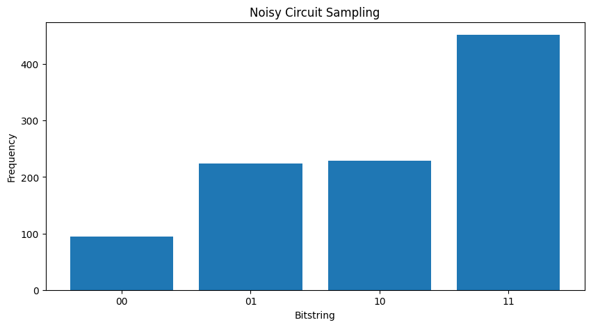
Comparing the two different \( \rho \) 's you can see that the noise has impacted the amplitudes of the state (and consequently sampling probabilities). In the noiseless case you would always expect to sample the \( |11\rangle \) state. But in the noisy state there is now a nonzero probability of sampling \( |00\rangle \) or \( |01\rangle \) or \( |10\rangle \) as well:

"""Sample from my_noisy_circuit."""
def plot_samples(circuit):
  samples = cirq.sample(circuit + cirq.measure(*circuit.all_qubits(), key='bits'), repetitions=1000)
  freqs, _ = np.histogram(samples.data['bits'], bins=[i+0.01 for i in range(-1,2** len(my_qubits))])
  plt.figure(figsize=(10,5))
  plt.title('Noisy Circuit Sampling')
  plt.xlabel('Bitstring')
  plt.ylabel('Frequency')
  plt.bar([i for i in range(2** len(my_qubits))], freqs, tick_label=['00','01','10','11'])

plot_samples(my_noisy_circuit)

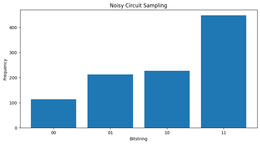
Without any noise you will always get \(|11\rangle\):

"""Sample from my_circuit."""
plot_samples(my_circuit)

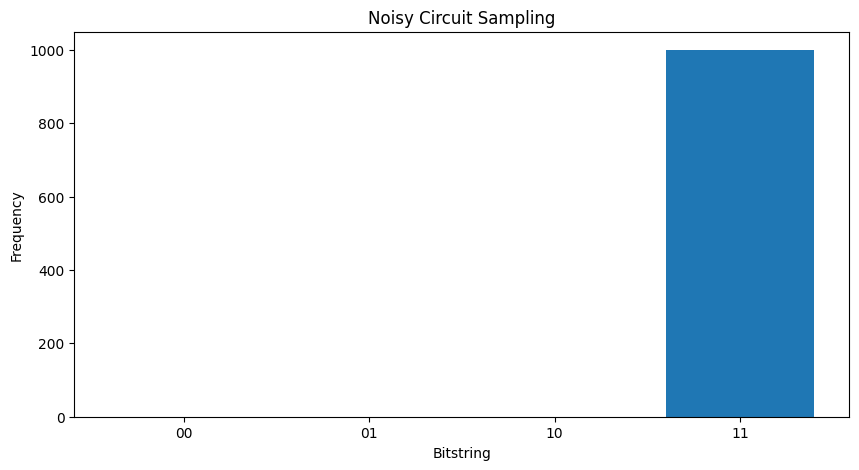
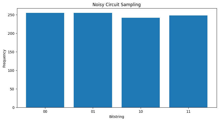
If you increase the noise a little further it will become harder and harder to distinguish the desired behavior (sampling \(|11\rangle\) ) from the noise:

my_really_noisy_circuit = make_noisy(my_circuit, 0.75)
plot_samples(my_really_noisy_circuit)

Note: Try experimenting with different channels in your circuit to generate noise. Common channels supported in both Cirq and TFQ can be found here

2. Basic noise in TFQ

With this understanding of how noise can impact circuit execution, you can explore how noise works in TFQ. TensorFlow Quantum uses monte-carlo / trajectory based simulation as an alternative to density matrix simulation. This is because the memory complexity of density matrix simulation limits large simulations to being <= 20 qubits with traditional full density matrix simulation methods. Monte-carlo / trajectory trades this cost in memory for additional cost in time. The backend='noisy' option available to all tfq.layers.Sample, tfq.layers.SampledExpectation and tfq.layers.Expectation (In the case of Expectation this does add a required repetitions parameter).

2.1 Noisy sampling in TFQ

To recreate the above plots using TFQ and trajectory simulation you can use tfq.layers.Sample

"""Draw bitstring samples from `my_noisy_circuit`"""
bitstrings = tfq.layers.Sample(backend='noisy')(my_noisy_circuit, repetitions=1000)

numeric_values = np.einsum('ijk,k->ij', bitstrings.to_tensor().numpy(), [1, 2])[0]
freqs, _ = np.histogram(numeric_values, bins=[i+0.01 for i in range(-1,2** len(my_qubits))])
plt.figure(figsize=(10,5))
plt.title('Noisy Circuit Sampling')
plt.xlabel('Bitstring')
plt.ylabel('Frequency')
plt.bar([i for i in range(2** len(my_qubits))], freqs, tick_label=['00','01','10','11'])

<BarContainer object of 4 artists>

2.2 Noisy sample based expectation

To do noisy sample based expectation calculation you can use tfq.layers.SampleExpectation:

some_observables = [cirq.X(my_qubits[0]), cirq.Z(my_qubits[0]), 3.0 * cirq.Y(my_qubits[1]) + 1]
some_observables

[cirq.X(cirq.GridQubit(0, 0)),
 cirq.Z(cirq.GridQubit(0, 0)),
 cirq.PauliSum(cirq.LinearDict({frozenset({(cirq.GridQubit(0, 1), cirq.Y)}): (3+0j), frozenset(): (1+0j)}))]

Compute the noiseless expectation estimates via sampling from the circuit:

noiseless_sampled_expectation = tfq.layers.SampledExpectation(backend='noiseless')(
    my_circuit, operators=some_observables, repetitions=10000
)
noiseless_sampled_expectation.numpy()

array([[-0.0066, -1.    ,  0.9892]], dtype=float32)

Compare those with the noisy versions:

noisy_sampled_expectation = tfq.layers.SampledExpectation(backend='noisy')(
    [my_noisy_circuit, my_really_noisy_circuit], operators=some_observables, repetitions=10000
)
noisy_sampled_expectation.numpy()

/tmpfs/src/tf_docs_env/lib/python3.9/site-packages/keras/src/initializers/initializers.py:120: UserWarning: The initializer RandomUniform is unseeded and being called multiple times, which will return identical values each time (even if the initializer is unseeded). Please update your code to provide a seed to the initializer, or avoid using the same initializer instance more than once.
  warnings.warn(
array([[-0.0034    , -0.34820002,  0.97959995],
       [-0.0118    ,  0.0042    ,  1.015     ]], dtype=float32)

You can see that the noise has particularly impacted the \(\langle \psi | Z | \psi \rangle\) accuracy, with my_really_noisy_circuit concentrating very quickly towards 0.

2.3 Noisy analytic expectation calculation

Doing noisy analytic expectation calculations is nearly identical to above:

noiseless_analytic_expectation = tfq.layers.Expectation(backend='noiseless')(
    my_circuit, operators=some_observables
)
noiseless_analytic_expectation.numpy()

array([[ 1.9106853e-15, -1.0000000e+00,  1.0000002e+00]], dtype=float32)

noisy_analytic_expectation = tfq.layers.Expectation(backend='noisy')(
    [my_noisy_circuit, my_really_noisy_circuit], operators=some_observables, repetitions=10000
)
noisy_analytic_expectation.numpy()

array([[ 1.9106853e-15, -3.3100003e-01,  1.0000000e+00],
       [ 1.9106855e-15,  5.0000018e-03,  1.0000000e+00]], dtype=float32)

3. Hybrid models and quantum data noise

Now that you have implemented some noisy circuit simulations in TFQ, you can experiment with how noise impacts quantum and hybrid quantum classical models, by comparing and contrasting their noisy vs noiseless performance. A good first check to see if a model or algorithm is robust to noise is to test under a circuit wide depolarizing model which looks something like this:

Where each time slice of the circuit (sometimes referred to as moment) has a depolarizing channel appended after each gate operation in that time slice. The depolarizing channel with apply one of \(\{X, Y, Z \}\) with probability \(p\) or apply nothing (keep the original operation) with probability \(1-p\).

3.1 Data

For this example you can use some prepared circuits in the tfq.datasets module as training data:

qubits = cirq.GridQubit.rect(1, 8)
circuits, labels, pauli_sums, _ = tfq.datasets.xxz_chain(qubits, 'closed')
circuits[0]

Downloading data from https://storage.googleapis.com/download.tensorflow.org/data/quantum/spin_systems/XXZ_chain.zip 
184449737/184449737 [==============================] - 2s 0us/step

Writing a small helper function will help to generate the data for the noisy vs noiseless case:

def get_data(qubits, depolarize_p=0.):
  """Return quantum data circuits and labels in `tf.Tensor` form."""
  circuits, labels, pauli_sums, _ = tfq.datasets.xxz_chain(qubits, 'closed')
  if depolarize_p >= 1e-5:
    circuits = [circuit.with_noise(cirq.depolarize(depolarize_p)) for circuit in circuits]
  tmp = list(zip(circuits, labels))
  random.shuffle(tmp)
  circuits_tensor = tfq.convert_to_tensor([x[0] for x in tmp])
  labels_tensor = tf.convert_to_tensor([x[1] for x in tmp])

  return circuits_tensor, labels_tensor

3.2 Define a model circuit

Now that you have quantum data in the form of circuits, you will need a circuit to model this data, like with the data you can write a helper function to generate this circuit optionally containing noise:

def modelling_circuit(qubits, depth, depolarize_p=0.):
  """A simple classifier circuit."""
  dim = len(qubits)
  ret = cirq.Circuit(cirq.H.on_each(*qubits))

  for i in range(depth):
    # Entangle layer.
    ret += cirq.Circuit(cirq.CX(q1, q2) for (q1, q2) in zip(qubits[::2], qubits[1::2]))
    ret += cirq.Circuit(cirq.CX(q1, q2) for (q1, q2) in zip(qubits[1::2], qubits[2::2]))
    # Learnable rotation layer.
    # i_params = sympy.symbols(f'layer-{i}-0:{dim}')
    param = sympy.Symbol(f'layer-{i}')
    single_qb = cirq.X
    if i % 2 == 1:
      single_qb = cirq.Y
    ret += cirq.Circuit(single_qb(q) ** param for q in qubits)

  if depolarize_p >= 1e-5:
    ret = ret.with_noise(cirq.depolarize(depolarize_p))

  return ret, [op(q) for q in qubits for op in [cirq.X, cirq.Y, cirq.Z]]

modelling_circuit(qubits, 3)[0]

3.3 Model building and training

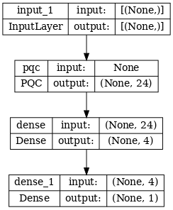
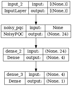
With your data and model circuit built, the final helper function you will need is one that can assemble both a noisy or a noiseless hybrid quantum tf.keras.Model:

def build_keras_model(qubits, depolarize_p=0.):
  """Prepare a noisy hybrid quantum classical Keras model."""
  spin_input = tf.keras.Input(shape=(), dtype=tf.dtypes.string)

  circuit_and_readout = modelling_circuit(qubits, 4, depolarize_p)
  if depolarize_p >= 1e-5:
    quantum_model = tfq.layers.NoisyPQC(*circuit_and_readout, sample_based=False, repetitions=10)(spin_input)
  else:
    quantum_model = tfq.layers.PQC(*circuit_and_readout)(spin_input)

  intermediate = tf.keras.layers.Dense(4, activation='sigmoid')(quantum_model)
  post_process = tf.keras.layers.Dense(1)(intermediate)

  return tf.keras.Model(inputs=[spin_input], outputs=[post_process])

4. Compare performance

4.1 Noiseless baseline

With your data generation and model building code, you can now compare and contrast model performance in the noiseless and noisy settings, first you can run a reference noiseless training:

training_histories = dict()
depolarize_p = 0.
n_epochs = 50
phase_classifier = build_keras_model(qubits, depolarize_p)

phase_classifier.compile(optimizer=tf.keras.optimizers.Adam(learning_rate=0.02),
                   loss=tf.keras.losses.BinaryCrossentropy(from_logits=True),
                   metrics=['accuracy'])


# Show the keras plot of the model
tf.keras.utils.plot_model(phase_classifier, show_shapes=True, dpi=70)

noiseless_data, noiseless_labels = get_data(qubits, depolarize_p)
training_histories['noiseless'] = phase_classifier.fit(x=noiseless_data,
                         y=noiseless_labels,
                         batch_size=16,
                         epochs=n_epochs,
                         validation_split=0.15,
                         verbose=1)

Epoch 1/50
4/4 [==============================] - 1s 129ms/step - loss: 0.6970 - accuracy: 0.4844 - val_loss: 0.6656 - val_accuracy: 0.4167
Epoch 2/50
4/4 [==============================] - 0s 62ms/step - loss: 0.6841 - accuracy: 0.4844 - val_loss: 0.6620 - val_accuracy: 0.4167
Epoch 3/50
4/4 [==============================] - 0s 66ms/step - loss: 0.6754 - accuracy: 0.4844 - val_loss: 0.6578 - val_accuracy: 0.4167
Epoch 4/50
4/4 [==============================] - 0s 62ms/step - loss: 0.6622 - accuracy: 0.4844 - val_loss: 0.6480 - val_accuracy: 0.4167
Epoch 5/50
4/4 [==============================] - 0s 63ms/step - loss: 0.6539 - accuracy: 0.4844 - val_loss: 0.6344 - val_accuracy: 0.4167
Epoch 6/50
4/4 [==============================] - 0s 62ms/step - loss: 0.6417 - accuracy: 0.4844 - val_loss: 0.6193 - val_accuracy: 0.4167
Epoch 7/50
4/4 [==============================] - 0s 61ms/step - loss: 0.6276 - accuracy: 0.4844 - val_loss: 0.6020 - val_accuracy: 0.4167
Epoch 8/50
4/4 [==============================] - 0s 60ms/step - loss: 0.6129 - accuracy: 0.4844 - val_loss: 0.5817 - val_accuracy: 0.4167
Epoch 9/50
4/4 [==============================] - 0s 61ms/step - loss: 0.5952 - accuracy: 0.5000 - val_loss: 0.5595 - val_accuracy: 0.6667
Epoch 10/50
4/4 [==============================] - 0s 60ms/step - loss: 0.5758 - accuracy: 0.6250 - val_loss: 0.5357 - val_accuracy: 0.7500
Epoch 11/50
4/4 [==============================] - 0s 61ms/step - loss: 0.5531 - accuracy: 0.6562 - val_loss: 0.5101 - val_accuracy: 0.9167
Epoch 12/50
4/4 [==============================] - 0s 59ms/step - loss: 0.5314 - accuracy: 0.7031 - val_loss: 0.4837 - val_accuracy: 0.9167
Epoch 13/50
4/4 [==============================] - 0s 59ms/step - loss: 0.5048 - accuracy: 0.7656 - val_loss: 0.4573 - val_accuracy: 0.9167
Epoch 14/50
4/4 [==============================] - 0s 59ms/step - loss: 0.4801 - accuracy: 0.7812 - val_loss: 0.4296 - val_accuracy: 0.9167
Epoch 15/50
4/4 [==============================] - 0s 61ms/step - loss: 0.4558 - accuracy: 0.7812 - val_loss: 0.4025 - val_accuracy: 0.9167
Epoch 16/50
4/4 [==============================] - 0s 60ms/step - loss: 0.4295 - accuracy: 0.8281 - val_loss: 0.3758 - val_accuracy: 0.9167
Epoch 17/50
4/4 [==============================] - 0s 59ms/step - loss: 0.4047 - accuracy: 0.8438 - val_loss: 0.3518 - val_accuracy: 1.0000
Epoch 18/50
4/4 [==============================] - 0s 60ms/step - loss: 0.3803 - accuracy: 0.8594 - val_loss: 0.3289 - val_accuracy: 1.0000
Epoch 19/50
4/4 [==============================] - 0s 61ms/step - loss: 0.3571 - accuracy: 0.8750 - val_loss: 0.3087 - val_accuracy: 1.0000
Epoch 20/50
4/4 [==============================] - 0s 60ms/step - loss: 0.3358 - accuracy: 0.9062 - val_loss: 0.2889 - val_accuracy: 1.0000
Epoch 21/50
4/4 [==============================] - 0s 60ms/step - loss: 0.3169 - accuracy: 0.9062 - val_loss: 0.2698 - val_accuracy: 1.0000
Epoch 22/50
4/4 [==============================] - 0s 60ms/step - loss: 0.2975 - accuracy: 0.9062 - val_loss: 0.2526 - val_accuracy: 1.0000
Epoch 23/50
4/4 [==============================] - 0s 60ms/step - loss: 0.2826 - accuracy: 0.9062 - val_loss: 0.2349 - val_accuracy: 1.0000
Epoch 24/50
4/4 [==============================] - 0s 59ms/step - loss: 0.2642 - accuracy: 0.9219 - val_loss: 0.2246 - val_accuracy: 1.0000
Epoch 25/50
4/4 [==============================] - 0s 60ms/step - loss: 0.2503 - accuracy: 0.9375 - val_loss: 0.2138 - val_accuracy: 1.0000
Epoch 26/50
4/4 [==============================] - 0s 60ms/step - loss: 0.2378 - accuracy: 0.9375 - val_loss: 0.2049 - val_accuracy: 1.0000
Epoch 27/50
4/4 [==============================] - 0s 59ms/step - loss: 0.2265 - accuracy: 0.9531 - val_loss: 0.1962 - val_accuracy: 1.0000
Epoch 28/50
4/4 [==============================] - 0s 59ms/step - loss: 0.2158 - accuracy: 0.9531 - val_loss: 0.1866 - val_accuracy: 1.0000
Epoch 29/50
4/4 [==============================] - 0s 59ms/step - loss: 0.2066 - accuracy: 0.9531 - val_loss: 0.1747 - val_accuracy: 1.0000
Epoch 30/50
4/4 [==============================] - 0s 60ms/step - loss: 0.1975 - accuracy: 0.9531 - val_loss: 0.1639 - val_accuracy: 1.0000
Epoch 31/50
4/4 [==============================] - 0s 59ms/step - loss: 0.1909 - accuracy: 0.9375 - val_loss: 0.1539 - val_accuracy: 1.0000
Epoch 32/50
4/4 [==============================] - 0s 59ms/step - loss: 0.1819 - accuracy: 0.9375 - val_loss: 0.1524 - val_accuracy: 1.0000
Epoch 33/50
4/4 [==============================] - 0s 59ms/step - loss: 0.1757 - accuracy: 0.9531 - val_loss: 0.1474 - val_accuracy: 1.0000
Epoch 34/50
4/4 [==============================] - 0s 59ms/step - loss: 0.1690 - accuracy: 0.9531 - val_loss: 0.1460 - val_accuracy: 1.0000
Epoch 35/50
4/4 [==============================] - 0s 58ms/step - loss: 0.1656 - accuracy: 0.9531 - val_loss: 0.1391 - val_accuracy: 1.0000
Epoch 36/50
4/4 [==============================] - 0s 59ms/step - loss: 0.1594 - accuracy: 0.9688 - val_loss: 0.1390 - val_accuracy: 1.0000
Epoch 37/50
4/4 [==============================] - 0s 59ms/step - loss: 0.1547 - accuracy: 0.9688 - val_loss: 0.1550 - val_accuracy: 1.0000
Epoch 38/50
4/4 [==============================] - 0s 60ms/step - loss: 0.1542 - accuracy: 0.9688 - val_loss: 0.1244 - val_accuracy: 1.0000
Epoch 39/50
4/4 [==============================] - 0s 59ms/step - loss: 0.1467 - accuracy: 0.9688 - val_loss: 0.1275 - val_accuracy: 1.0000
Epoch 40/50
4/4 [==============================] - 0s 60ms/step - loss: 0.1485 - accuracy: 0.9688 - val_loss: 0.1254 - val_accuracy: 1.0000
Epoch 41/50
4/4 [==============================] - 0s 59ms/step - loss: 0.1421 - accuracy: 0.9531 - val_loss: 0.1239 - val_accuracy: 1.0000
Epoch 42/50
4/4 [==============================] - 0s 59ms/step - loss: 0.1453 - accuracy: 0.9844 - val_loss: 0.1243 - val_accuracy: 1.0000
Epoch 43/50
4/4 [==============================] - 0s 59ms/step - loss: 0.1333 - accuracy: 0.9844 - val_loss: 0.1065 - val_accuracy: 1.0000
Epoch 44/50
4/4 [==============================] - 0s 58ms/step - loss: 0.1361 - accuracy: 0.9375 - val_loss: 0.0930 - val_accuracy: 1.0000
Epoch 45/50
4/4 [==============================] - 0s 59ms/step - loss: 0.1303 - accuracy: 0.9531 - val_loss: 0.1082 - val_accuracy: 1.0000
Epoch 46/50
4/4 [==============================] - 0s 60ms/step - loss: 0.1237 - accuracy: 0.9688 - val_loss: 0.1091 - val_accuracy: 1.0000
Epoch 47/50
4/4 [==============================] - 0s 59ms/step - loss: 0.1202 - accuracy: 0.9844 - val_loss: 0.1053 - val_accuracy: 1.0000
Epoch 48/50
4/4 [==============================] - 0s 59ms/step - loss: 0.1169 - accuracy: 0.9688 - val_loss: 0.0991 - val_accuracy: 1.0000
Epoch 49/50
4/4 [==============================] - 0s 59ms/step - loss: 0.1142 - accuracy: 0.9688 - val_loss: 0.0982 - val_accuracy: 1.0000
Epoch 50/50
4/4 [==============================] - 0s 61ms/step - loss: 0.1129 - accuracy: 0.9688 - val_loss: 0.1005 - val_accuracy: 1.0000

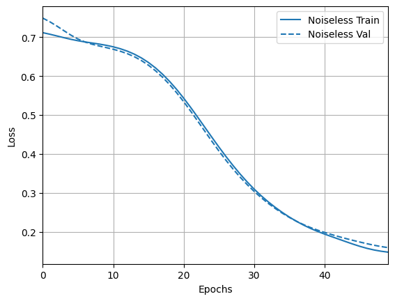
And explore the results and accuracy:

loss_plotter = tfdocs.plots.HistoryPlotter(metric = 'loss', smoothing_std=10)
loss_plotter.plot(training_histories)

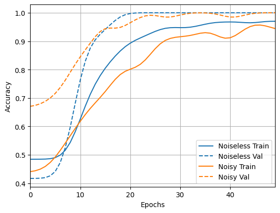
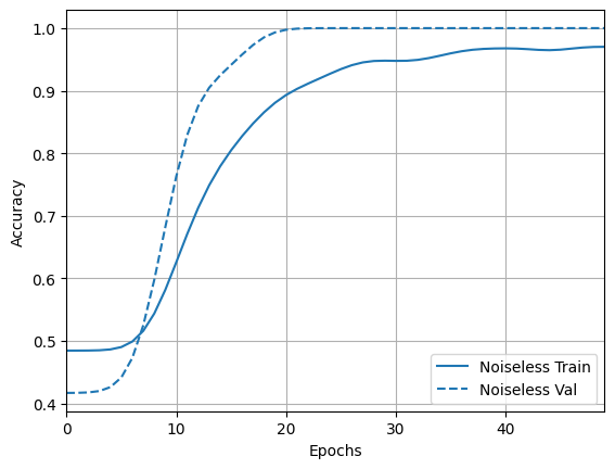
acc_plotter = tfdocs.plots.HistoryPlotter(metric = 'accuracy', smoothing_std=10)
acc_plotter.plot(training_histories)

4.2 Noisy comparison

Now you can build a new model with noisy structure and compare to the above, the code is nearly identical:

depolarize_p = 0.001
n_epochs = 50
noisy_phase_classifier = build_keras_model(qubits, depolarize_p)

noisy_phase_classifier.compile(optimizer=tf.keras.optimizers.Adam(learning_rate=0.02),
                   loss=tf.keras.losses.BinaryCrossentropy(from_logits=True),
                   metrics=['accuracy'])


# Show the keras plot of the model
tf.keras.utils.plot_model(noisy_phase_classifier, show_shapes=True, dpi=70)

Note: in the model diagram there is now a tfq.layers.NoisyPQC instead of a tfq.layers.PQC since the depolarization probability is no longer zero. Training will take significantly longer since noisy simulation is far more expensive than noiseless.

noisy_data, noisy_labels = get_data(qubits, depolarize_p)
training_histories['noisy'] = noisy_phase_classifier.fit(x=noisy_data,
                         y=noisy_labels,
                         batch_size=16,
                         epochs=n_epochs,
                         validation_split=0.15,
                         verbose=1)

Epoch 1/50
4/4 [==============================] - 9s 1s/step - loss: 0.6851 - accuracy: 0.4375 - val_loss: 0.6770 - val_accuracy: 0.6667
Epoch 2/50
4/4 [==============================] - 5s 1s/step - loss: 0.6696 - accuracy: 0.4375 - val_loss: 0.6996 - val_accuracy: 0.6667
Epoch 3/50
4/4 [==============================] - 5s 1s/step - loss: 0.6609 - accuracy: 0.4375 - val_loss: 0.7085 - val_accuracy: 0.6667
Epoch 4/50
4/4 [==============================] - 5s 1s/step - loss: 0.6501 - accuracy: 0.4375 - val_loss: 0.7097 - val_accuracy: 0.6667
Epoch 5/50
4/4 [==============================] - 5s 1s/step - loss: 0.6461 - accuracy: 0.4844 - val_loss: 0.6984 - val_accuracy: 0.7500
Epoch 6/50
4/4 [==============================] - 5s 1s/step - loss: 0.6379 - accuracy: 0.4844 - val_loss: 0.6806 - val_accuracy: 0.6667
Epoch 7/50
4/4 [==============================] - 5s 1s/step - loss: 0.6281 - accuracy: 0.5156 - val_loss: 0.6689 - val_accuracy: 0.7500
Epoch 8/50
4/4 [==============================] - 5s 1s/step - loss: 0.6176 - accuracy: 0.5781 - val_loss: 0.6502 - val_accuracy: 0.7500
Epoch 9/50
4/4 [==============================] - 5s 1s/step - loss: 0.6082 - accuracy: 0.5938 - val_loss: 0.6304 - val_accuracy: 0.8333
Epoch 10/50
4/4 [==============================] - 5s 1s/step - loss: 0.5994 - accuracy: 0.5781 - val_loss: 0.6079 - val_accuracy: 0.8333
Epoch 11/50
4/4 [==============================] - 5s 1s/step - loss: 0.5889 - accuracy: 0.6250 - val_loss: 0.5922 - val_accuracy: 0.9167
Epoch 12/50
4/4 [==============================] - 5s 1s/step - loss: 0.5698 - accuracy: 0.6875 - val_loss: 0.5856 - val_accuracy: 0.8333
Epoch 13/50
4/4 [==============================] - 5s 1s/step - loss: 0.5624 - accuracy: 0.6875 - val_loss: 0.5666 - val_accuracy: 0.8333
Epoch 14/50
4/4 [==============================] - 5s 1s/step - loss: 0.5419 - accuracy: 0.6719 - val_loss: 0.5141 - val_accuracy: 1.0000
Epoch 15/50
4/4 [==============================] - 5s 1s/step - loss: 0.5321 - accuracy: 0.7188 - val_loss: 0.5024 - val_accuracy: 1.0000
Epoch 16/50
4/4 [==============================] - 5s 1s/step - loss: 0.5228 - accuracy: 0.6875 - val_loss: 0.4970 - val_accuracy: 1.0000
Epoch 17/50
4/4 [==============================] - 5s 1s/step - loss: 0.4946 - accuracy: 0.7812 - val_loss: 0.4924 - val_accuracy: 0.9167
Epoch 18/50
4/4 [==============================] - 5s 1s/step - loss: 0.4873 - accuracy: 0.7969 - val_loss: 0.4714 - val_accuracy: 0.8333
Epoch 19/50
4/4 [==============================] - 5s 1s/step - loss: 0.4708 - accuracy: 0.8281 - val_loss: 0.4329 - val_accuracy: 1.0000
Epoch 20/50
4/4 [==============================] - 5s 1s/step - loss: 0.4628 - accuracy: 0.7969 - val_loss: 0.3888 - val_accuracy: 1.0000
Epoch 21/50
4/4 [==============================] - 5s 1s/step - loss: 0.4419 - accuracy: 0.7969 - val_loss: 0.3807 - val_accuracy: 0.9167
Epoch 22/50
4/4 [==============================] - 5s 1s/step - loss: 0.4307 - accuracy: 0.7969 - val_loss: 0.3384 - val_accuracy: 1.0000
Epoch 23/50
4/4 [==============================] - 5s 1s/step - loss: 0.4010 - accuracy: 0.7969 - val_loss: 0.3665 - val_accuracy: 1.0000
Epoch 24/50
4/4 [==============================] - 5s 1s/step - loss: 0.3922 - accuracy: 0.8125 - val_loss: 0.3271 - val_accuracy: 1.0000
Epoch 25/50
4/4 [==============================] - 5s 1s/step - loss: 0.3638 - accuracy: 0.8906 - val_loss: 0.3407 - val_accuracy: 1.0000
Epoch 26/50
4/4 [==============================] - 5s 1s/step - loss: 0.3456 - accuracy: 0.9062 - val_loss: 0.2935 - val_accuracy: 1.0000
Epoch 27/50
4/4 [==============================] - 5s 1s/step - loss: 0.3580 - accuracy: 0.9219 - val_loss: 0.2527 - val_accuracy: 1.0000
Epoch 28/50
4/4 [==============================] - 5s 1s/step - loss: 0.3323 - accuracy: 0.9062 - val_loss: 0.3143 - val_accuracy: 0.9167
Epoch 29/50
4/4 [==============================] - 5s 1s/step - loss: 0.3380 - accuracy: 0.9062 - val_loss: 0.3100 - val_accuracy: 1.0000
Epoch 30/50
4/4 [==============================] - 5s 1s/step - loss: 0.2893 - accuracy: 0.9375 - val_loss: 0.2266 - val_accuracy: 1.0000
Epoch 31/50
4/4 [==============================] - 5s 1s/step - loss: 0.3008 - accuracy: 0.9062 - val_loss: 0.2205 - val_accuracy: 1.0000
Epoch 32/50
4/4 [==============================] - 5s 1s/step - loss: 0.2806 - accuracy: 0.9062 - val_loss: 0.2191 - val_accuracy: 1.0000
Epoch 33/50
4/4 [==============================] - 5s 1s/step - loss: 0.2657 - accuracy: 0.9219 - val_loss: 0.1817 - val_accuracy: 1.0000
Epoch 34/50
4/4 [==============================] - 5s 1s/step - loss: 0.2722 - accuracy: 0.9375 - val_loss: 0.2123 - val_accuracy: 1.0000
Epoch 35/50
4/4 [==============================] - 5s 1s/step - loss: 0.2790 - accuracy: 0.8906 - val_loss: 0.1979 - val_accuracy: 1.0000
Epoch 36/50
4/4 [==============================] - 5s 1s/step - loss: 0.2423 - accuracy: 0.9844 - val_loss: 0.2043 - val_accuracy: 1.0000
Epoch 37/50
4/4 [==============================] - 5s 1s/step - loss: 0.2493 - accuracy: 0.9688 - val_loss: 0.1863 - val_accuracy: 1.0000
Epoch 38/50
4/4 [==============================] - 5s 1s/step - loss: 0.2604 - accuracy: 0.8906 - val_loss: 0.1987 - val_accuracy: 1.0000
Epoch 39/50
4/4 [==============================] - 5s 1s/step - loss: 0.2329 - accuracy: 0.8906 - val_loss: 0.1580 - val_accuracy: 1.0000
Epoch 40/50
4/4 [==============================] - 5s 1s/step - loss: 0.2420 - accuracy: 0.8906 - val_loss: 0.1558 - val_accuracy: 1.0000
Epoch 41/50
4/4 [==============================] - 5s 1s/step - loss: 0.2384 - accuracy: 0.8750 - val_loss: 0.2039 - val_accuracy: 0.9167
Epoch 42/50
4/4 [==============================] - 5s 1s/step - loss: 0.2396 - accuracy: 0.9375 - val_loss: 0.1347 - val_accuracy: 1.0000
Epoch 43/50
4/4 [==============================] - 5s 1s/step - loss: 0.2038 - accuracy: 0.9531 - val_loss: 0.1266 - val_accuracy: 1.0000
Epoch 44/50
4/4 [==============================] - 5s 1s/step - loss: 0.2223 - accuracy: 0.9531 - val_loss: 0.1334 - val_accuracy: 1.0000
Epoch 45/50
4/4 [==============================] - 5s 1s/step - loss: 0.2050 - accuracy: 0.9688 - val_loss: 0.1155 - val_accuracy: 1.0000
Epoch 46/50
4/4 [==============================] - 5s 1s/step - loss: 0.1815 - accuracy: 0.9531 - val_loss: 0.1298 - val_accuracy: 1.0000
Epoch 47/50
4/4 [==============================] - 5s 1s/step - loss: 0.1666 - accuracy: 1.0000 - val_loss: 0.0986 - val_accuracy: 1.0000
Epoch 48/50
4/4 [==============================] - 5s 1s/step - loss: 0.1885 - accuracy: 0.9375 - val_loss: 0.0958 - val_accuracy: 1.0000
Epoch 49/50
4/4 [==============================] - 5s 1s/step - loss: 0.1865 - accuracy: 0.9219 - val_loss: 0.1410 - val_accuracy: 1.0000
Epoch 50/50
4/4 [==============================] - 5s 1s/step - loss: 0.1887 - accuracy: 0.9375 - val_loss: 0.1307 - val_accuracy: 1.0000

loss_plotter.plot(training_histories)

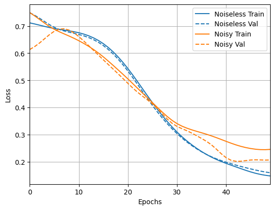
acc_plotter.plot(training_histories)

Success: The noisy model still managed to train under some mild depolarization noise. Try experimenting with different noise models to see how and when training might fail. Also look out for noisy functionality under tfq.layers and tfq.noise.