TensorFlow Addons Optimizers: CyclicalLearningRate

Overview

This tutorial demonstrates the use of Cyclical Learning Rate from the Addons package.

Cyclical Learning Rates

It has been shown it is beneficial to adjust the learning rate as training progresses for a neural network. It has manifold benefits ranging from saddle point recovery to preventing numerical instabilities that may arise during backpropagation. But how does one know how much to adjust with respect to a particular training timestamp? In 2015, Leslie Smith noticed that you would want to increase the learning rate to traverse faster across the loss landscape but you would also want to reduce the learning rate when approaching convergence. To realize this idea, he proposed Cyclical Learning Rates (CLR) where you would adjust the learning rate with respect to the cycles of a function. For a visual demonstration, you can check out this blog. CLR is now available as a TensorFlow API. For more details, check out the original paper here.

Setup

pip install -q -U tensorflow_addons

from tensorflow.keras import layers
import tensorflow_addons as tfa
import tensorflow as tf

import numpy as np
import matplotlib.pyplot as plt

tf.random.set_seed(42)
np.random.seed(42)

Load and prepare dataset

(x_train, y_train), (x_test, y_test) = tf.keras.datasets.fashion_mnist.load_data()

x_train = np.expand_dims(x_train, -1)
x_test = np.expand_dims(x_test, -1)

Define hyperparameters

BATCH_SIZE = 64
EPOCHS = 10
INIT_LR = 1e-4
MAX_LR = 1e-2

Define model building and model training utilities

def get_training_model():
    model = tf.keras.Sequential(
        [
            layers.InputLayer((28, 28, 1)),
            layers.experimental.preprocessing.Rescaling(scale=1./255),
            layers.Conv2D(16, (5, 5), activation="relu"),
            layers.MaxPooling2D(pool_size=(2, 2)),
            layers.Conv2D(32, (5, 5), activation="relu"),
            layers.MaxPooling2D(pool_size=(2, 2)),
            layers.SpatialDropout2D(0.2),
            layers.GlobalAvgPool2D(),
            layers.Dense(128, activation="relu"),
            layers.Dense(10, activation="softmax"),
        ]
    )
    return model

def train_model(model, optimizer):
    model.compile(loss="sparse_categorical_crossentropy", optimizer=optimizer,
                       metrics=["accuracy"])
    history = model.fit(x_train,
        y_train,
        batch_size=BATCH_SIZE,
        validation_data=(x_test, y_test),
        epochs=EPOCHS)
    return history

In the interest of reproducibility, the initial model weights are serialized which you will be using to conduct our experiments.

initial_model = get_training_model()
initial_model.save("initial_model")

WARNING:tensorflow:Compiled the loaded model, but the compiled metrics have yet to be built. `model.compile_metrics` will be empty until you train or evaluate the model.
WARNING:absl:Found untraced functions such as _jit_compiled_convolution_op, _jit_compiled_convolution_op while saving (showing 2 of 2). These functions will not be directly callable after loading.
INFO:tensorflow:Assets written to: initial_model/assets
INFO:tensorflow:Assets written to: initial_model/assets

Train a model without CLR

standard_model = tf.keras.models.load_model("initial_model")
no_clr_history = train_model(standard_model, optimizer="sgd")

WARNING:tensorflow:No training configuration found in save file, so the model was *not* compiled. Compile it manually.
WARNING:tensorflow:No training configuration found in save file, so the model was *not* compiled. Compile it manually.
Epoch 1/10
938/938 [==============================] - 4s 3ms/step - loss: 2.2088 - accuracy: 0.2182 - val_loss: 1.7579 - val_accuracy: 0.4108
Epoch 2/10
938/938 [==============================] - 3s 3ms/step - loss: 1.2954 - accuracy: 0.5133 - val_loss: 0.9588 - val_accuracy: 0.6488
Epoch 3/10
938/938 [==============================] - 3s 3ms/step - loss: 1.0101 - accuracy: 0.6188 - val_loss: 0.9154 - val_accuracy: 0.6586
Epoch 4/10
938/938 [==============================] - 3s 3ms/step - loss: 0.9275 - accuracy: 0.6568 - val_loss: 0.8503 - val_accuracy: 0.7002
Epoch 5/10
938/938 [==============================] - 3s 3ms/step - loss: 0.8859 - accuracy: 0.6720 - val_loss: 0.8415 - val_accuracy: 0.6665
Epoch 6/10
938/938 [==============================] - 3s 3ms/step - loss: 0.8484 - accuracy: 0.6849 - val_loss: 0.7979 - val_accuracy: 0.6826
Epoch 7/10
938/938 [==============================] - 3s 3ms/step - loss: 0.8221 - accuracy: 0.6940 - val_loss: 0.7621 - val_accuracy: 0.6996
Epoch 8/10
938/938 [==============================] - 3s 3ms/step - loss: 0.7998 - accuracy: 0.7010 - val_loss: 0.7274 - val_accuracy: 0.7279
Epoch 9/10
938/938 [==============================] - 3s 3ms/step - loss: 0.7834 - accuracy: 0.7063 - val_loss: 0.7159 - val_accuracy: 0.7446
Epoch 10/10
938/938 [==============================] - 3s 3ms/step - loss: 0.7640 - accuracy: 0.7134 - val_loss: 0.7025 - val_accuracy: 0.7466

Define CLR schedule

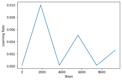
The tfa.optimizers.CyclicalLearningRate module return a direct schedule that can be passed to an optimizer. The schedule takes a step as its input and outputs a value calculated using CLR formula as laid out in the paper.

steps_per_epoch = len(x_train) // BATCH_SIZE
clr = tfa.optimizers.CyclicalLearningRate(initial_learning_rate=INIT_LR,
    maximal_learning_rate=MAX_LR,
    scale_fn=lambda x: 1/(2.**(x-1)),
    step_size=2 * steps_per_epoch
)
optimizer = tf.keras.optimizers.SGD(clr)

Here, you specify the lower and upper bounds of the learning rate and the schedule will oscillate in between that range ([1e-4, 1e-2] in this case). scale_fn is used to define the function that would scale up and scale down the learning rate within a given cycle. step_size defines the duration of a single cycle. A step_size of 2 means you need a total of 4 iterations to complete one cycle. The recommended value for step_size is as follows:

factor * steps_per_epoch where factor lies within the [2, 8] range.

In the same CLR paper, Leslie also presented a simple and elegant method to choose the bounds for learning rate. You are encouraged to check it out as well. This blog post provides a nice introduction to the method.

Below, you visualize how the clr schedule looks like.

step = np.arange(0, EPOCHS * steps_per_epoch)
lr = clr(step)
plt.plot(step, lr)
plt.xlabel("Steps")
plt.ylabel("Learning Rate")
plt.show()

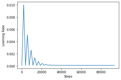
In order to better visualize the effect of CLR, you can plot the schedule with an increased number of steps.

step = np.arange(0, 100 * steps_per_epoch)
lr = clr(step)
plt.plot(step, lr)
plt.xlabel("Steps")
plt.ylabel("Learning Rate")
plt.show()

The function you are using in this tutorial is referred to as the triangular2 method in the CLR paper. There are other two functions there were explored namely triangular and exp (short for exponential).

Train a model with CLR

clr_model = tf.keras.models.load_model("initial_model")
clr_history = train_model(clr_model, optimizer=optimizer)

WARNING:tensorflow:No training configuration found in save file, so the model was *not* compiled. Compile it manually.
WARNING:tensorflow:No training configuration found in save file, so the model was *not* compiled. Compile it manually.
Epoch 1/10
938/938 [==============================] - 3s 3ms/step - loss: 2.3005 - accuracy: 0.1165 - val_loss: 2.2852 - val_accuracy: 0.2375
Epoch 2/10
938/938 [==============================] - 3s 3ms/step - loss: 2.1930 - accuracy: 0.2397 - val_loss: 1.7384 - val_accuracy: 0.4520
Epoch 3/10
938/938 [==============================] - 3s 3ms/step - loss: 1.3132 - accuracy: 0.5055 - val_loss: 1.0109 - val_accuracy: 0.6493
Epoch 4/10
938/938 [==============================] - 3s 3ms/step - loss: 1.0748 - accuracy: 0.5930 - val_loss: 0.9493 - val_accuracy: 0.6625
Epoch 5/10
938/938 [==============================] - 3s 3ms/step - loss: 1.0530 - accuracy: 0.6028 - val_loss: 0.9441 - val_accuracy: 0.6523
Epoch 6/10
938/938 [==============================] - 3s 3ms/step - loss: 1.0199 - accuracy: 0.6172 - val_loss: 0.9101 - val_accuracy: 0.6617
Epoch 7/10
938/938 [==============================] - 3s 3ms/step - loss: 0.9780 - accuracy: 0.6345 - val_loss: 0.8785 - val_accuracy: 0.6755
Epoch 8/10
938/938 [==============================] - 3s 3ms/step - loss: 0.9536 - accuracy: 0.6486 - val_loss: 0.8666 - val_accuracy: 0.6907
Epoch 9/10
938/938 [==============================] - 3s 3ms/step - loss: 0.9512 - accuracy: 0.6496 - val_loss: 0.8690 - val_accuracy: 0.6868
Epoch 10/10
938/938 [==============================] - 3s 3ms/step - loss: 0.9425 - accuracy: 0.6526 - val_loss: 0.8570 - val_accuracy: 0.6921

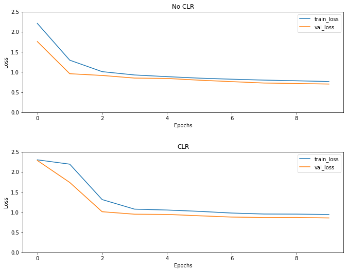
As expected the loss starts higher than the usual and then it stabilizes as the cycles progress. You can confirm this visually with the plots below.

Visualize losses

(fig, ax) = plt.subplots(2, 1, figsize=(10, 8))

ax[0].plot(no_clr_history.history["loss"], label="train_loss")
ax[0].plot(no_clr_history.history["val_loss"], label="val_loss")
ax[0].set_title("No CLR")
ax[0].set_xlabel("Epochs")
ax[0].set_ylabel("Loss")
ax[0].set_ylim([0, 2.5])
ax[0].legend()

ax[1].plot(clr_history.history["loss"], label="train_loss")
ax[1].plot(clr_history.history["val_loss"], label="val_loss")
ax[1].set_title("CLR")
ax[1].set_xlabel("Epochs")
ax[1].set_ylabel("Loss")
ax[1].set_ylim([0, 2.5])
ax[1].legend()

fig.tight_layout(pad=3.0)
fig.show()

Even though for this toy example, you did not see the effects of CLR much but be noted that it is one of the main ingredients behind Super Convergence and can have a really good impact when training in large-scale settings.