
|
|
|
 View on GitHub View on GitHub
|
|
This tutorial shows how to "warm-start" training using the tf.keras.utils.warmstart_embedding_matrix API for text sentiment classification when changing vocabulary.
You will begin by training a simple Keras model with a base vocabulary, and then, after updating the vocabulary, continue training the model. This is referred to as "warm-start" training, for which you'll need to remap the text-embedding matrix for the new vocabulary.
Embedding matrix
Embeddings provide a way to use an efficient, dense representation in which similar vocabulary tokens have a similar encoding. They are trainable parameters (weights learned by the model during training, in the same way a model learns weights for a dense layer). It is common to have embeddings that are 8-dimensional for small datasets, and up to 1024-dimensions when working with large datasets. A higher dimensional embedding can capture fine-grained relationships between words, but can take more data to learn.
Vocabulary
The set of unique words is referred to as the vocabulary. To build a text model you need to choose a fixed vocabulary. Typically you build the vocabulary from the most common words in a dataset. The vocabulary allows us to represent each piece of text by a sequence of ID's that you can lookup in the embedding matrix. Vocabulary allows us to represent each piece of text by the specific words that appear in it.
Why warm-start an embedding matrix?
A model is trained with a set of embeddings that represents a given vocabulary. If the model needs to be updated or improved you can train to convergence significantly faster by reusing weights from a previous run. Using the embedding matrix from a previous run is more difficult. The problem is that any change to the vocabulary invalidates the word to id mapping.
The tf.keras.utils.warmstart_embedding_matrix solves this problem by creating an embedding matrix for a new vocabulary from an embedding matrix from a base vocabulary. Where a word exists in both vocabularies the base embedding vector is copied into the correct location in the new embedding matrix. This allows you to warm-start training after any change in the size or order of the vocabulary.
Setup
pip install --pre -U "tensorflow>2.10" # Requires 2.11import io
import numpy as np
import os
import re
import shutil
import string
import tensorflow as tf
from tensorflow.keras import Model
from tensorflow.keras.layers import Dense, Embedding, GlobalAveragePooling1D
from tensorflow.keras.layers import TextVectorization
Load the dataset
The tutorial uses the Large Movie Review Dataset. You will train a sentiment classifier model on this dataset and in the process learn embeddings from scratch. Refer to the Loading text tutorial to learn more.
Download the dataset using Keras file utility and review the directories.
url = "https://ai.stanford.edu/~amaas/data/sentiment/aclImdb_v1.tar.gz"

dataset = tf.keras.utils.get_file(
    "aclImdb_v1.tar.gz", url, untar=True, cache_dir=".", cache_subdir=""
)

dataset_dir = os.path.join(os.path.dirname(dataset), "aclImdb")
os.listdir(dataset_dir)
The train/ directory has pos and neg folders with movie reviews labeled as positive and negative respectively. You will use reviews from pos and neg folders to train a binary classification model.
train_dir = os.path.join(dataset_dir, "train")
os.listdir(train_dir)
The train directory also contains additional folders which should be removed before creating the training set.
remove_dir = os.path.join(train_dir, "unsup")
shutil.rmtree(remove_dir)
Next, create a tf.data.Dataset using tf.keras.utils.text_dataset_from_directory. You can read more about using this utility in this text classification tutorial.
Use the train directory to create the training and validation sets with a split of 20% for validation.
batch_size = 1024
seed = 123
train_ds = tf.keras.utils.text_dataset_from_directory(
    "aclImdb/train",
    batch_size=batch_size,
    validation_split=0.2,
    subset="training",
    seed=seed,
)
val_ds = tf.keras.utils.text_dataset_from_directory(
    "aclImdb/train",
    batch_size=batch_size,
    validation_split=0.2,
    subset="validation",
    seed=seed,
)
Configure the dataset for performance
You can learn more about Dataset.cache and Dataset.prefetch, as well as how to cache data to disk in the data performance guide.
AUTOTUNE = tf.data.AUTOTUNE

train_ds = train_ds.cache().prefetch(buffer_size=AUTOTUNE)
val_ds = val_ds.cache().prefetch(buffer_size=AUTOTUNE)
Text preprocessing
Next, define the dataset preprocessing steps required for your sentiment classification model. Initialize a layers.TextVectorization layer with the desired parameters to vectorize movie reviews. You can learn more about using this layer in the Text Classification tutorial.
# Create a custom standardization function to strip HTML break tags '<br />'.
def custom_standardization(input_data):
    lowercase = tf.strings.lower(input_data)
    stripped_html = tf.strings.regex_replace(lowercase, "<br />", " ")
    return tf.strings.regex_replace(
        stripped_html, "[%s]" % re.escape(string.punctuation), ""
    )


# Vocabulary size and number of words in a sequence.
vocab_size = 10000
sequence_length = 100

# Use the text vectorization layer to normalize, split, and map strings to
# integers. Note that the layer uses the custom standardization defined above.
# Set maximum_sequence length as all samples are not of the same length.
vectorize_layer = TextVectorization(
    standardize=custom_standardization,
    max_tokens=vocab_size,
    output_mode="int",
    output_sequence_length=sequence_length,
)

# Make a text-only dataset (no labels) and call `Dataset.adapt` to build the
# vocabulary.
text_ds = train_ds.map(lambda x, y: x)
vectorize_layer.adapt(text_ds)
Create a classification model
Use the Keras Sequential API to define the sentiment classification model.
embedding_dim = 16
text_embedding = Embedding(vocab_size, embedding_dim, name="embedding")
text_input = tf.keras.Sequential(
    [vectorize_layer, text_embedding], name="text_input"
)
classifier_head = tf.keras.Sequential(
    [GlobalAveragePooling1D(), Dense(16, activation="relu"), Dense(1)],
    name="classifier_head",
)

model = tf.keras.Sequential([text_input, classifier_head])
Compile and train the model
You will use TensorBoard to visualize metrics including loss and accuracy. Create a tf.keras.callbacks.TensorBoard.
tensorboard_callback = tf.keras.callbacks.TensorBoard(log_dir="logs")
Compile and train the model using the Adam optimizer and BinaryCrossentropy loss.
model.compile(
    optimizer="adam",
    loss=tf.keras.losses.BinaryCrossentropy(from_logits=True),
    metrics=["accuracy"],
)
model.fit(
    train_ds,
    validation_data=val_ds,
    epochs=15,
    callbacks=[tensorboard_callback],
)
With this approach the model reaches a validation accuracy of around 85%
You can look into the model summary to learn more about each layer of the model.
model.summary()
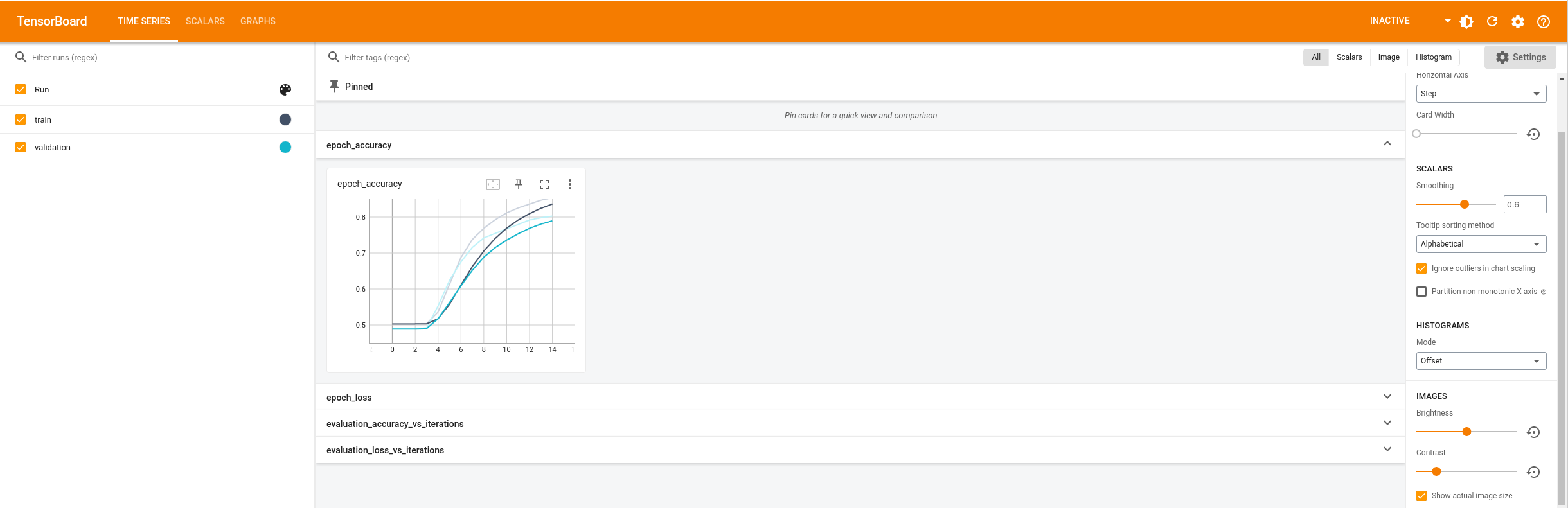
Visualize the model metrics in TensorBoard.
# docs_infra: no_execute
%load_ext tensorboard
%tensorboard --logdir logs
Vocabulary remapping
Now you're going to update the vocabulary and continue with warm-started training.
First, get the base vocabulary and embedding matrix.
embedding_weights_base = (
    model.get_layer("text_input").get_layer("embedding").embeddings
)
vocab_base = vectorize_layer.get_vocabulary()
Define a new vectorization layer to generate a new bigger vocabulary
# Vocabulary size and number of words in a sequence.
vocab_size_new = 10200
sequence_length = 100

vectorize_layer_new = TextVectorization(
    standardize=custom_standardization,
    max_tokens=vocab_size_new,
    output_mode="int",
    output_sequence_length=sequence_length,
)

# Make a text-only dataset (no labels) and call adapt to build the vocabulary.
text_ds = train_ds.map(lambda x, y: x)
vectorize_layer_new.adapt(text_ds)

# Get the new vocabulary
vocab_new = vectorize_layer_new.get_vocabulary()
# View the new vocabulary tokens that weren't in `vocab_base`
set(vocab_base) ^ set(vocab_new)
Generate updated embeddings using the keras.utils.warmstart_embedding_matrix util.
# Generate the updated embedding matrix
updated_embedding = tf.keras.utils.warmstart_embedding_matrix(
    base_vocabulary=vocab_base,
    new_vocabulary=vocab_new,
    base_embeddings=embedding_weights_base,
    new_embeddings_initializer="uniform",
)
# Update the model variable
updated_embedding_variable = tf.Variable(updated_embedding)
OR
If you have an embedding matrix which you would like to initialize the new embedding matrix with, use keras.initializers.Constant as new_embeddings initializer. Copy the following block to a code cell to try this out.
This would be helpful when you have a better embedding matrix initialization for new words in vocab.
# generate updated embedding matrix
new_embedding = np.random.rand(len(vocab_new), 16)
updated_embedding = tf.keras.utils.warmstart_embedding_matrix(
            base_vocabulary=vocab_base,
            new_vocabulary=vocab_new,
            base_embeddings=embedding_weights_base,
            new_embeddings_initializer=tf.keras.initializers.Constant(
                new_embedding
            )
        )
# update model variable
updated_embedding_variable = tf.Variable(updated_embedding)
Verify if the embedding matrix's shape has changed to reflect the new vocabulary.
updated_embedding_variable.shape
Now that you have the updated embedding matrix, the next step is to update the layer weights.
text_embedding_layer_new = Embedding(
    vectorize_layer_new.vocabulary_size(), embedding_dim, name="embedding"
)
text_embedding_layer_new.build(input_shape=[None])
text_embedding_layer_new.embeddings.assign(updated_embedding)
text_input_new = tf.keras.Sequential(
    [vectorize_layer_new, text_embedding_layer_new], name="text_input_new"
)
text_input_new.summary()

# Verify the shape of updated weights
# The new weights shape should reflect the new vocabulary size
text_input_new.get_layer("embedding").embeddings.shape
Modify the model architecture to use the new text vectorization layer.
You can also load the model from a checkpoint and update the model architecture as shown below.
warm_started_model = tf.keras.Sequential([text_input_new, classifier_head])
warm_started_model.summary()
You have successfully updated the model to accept a new vocabulary. The embedding layer is updated to map old vocabulary words to old embeddings and initialize embeddings for new vocabulary words to be learnt. The learned weights of the rest of the model will remain the same. The model is warm-started to continue to train from where it left off previously.
You can now verify that the remapping worked. Get the index of the vocabulary word "the" that is present both in base and new vocabulary and compare the embedding values. They should be equal.
# New vocab words
base_vocab_index = vectorize_layer("the")[0]
new_vocab_index = vectorize_layer_new("the")[0]
print(
    warm_started_model.get_layer("text_input_new").get_layer("embedding")(
        new_vocab_index
    )
    == embedding_weights_base[base_vocab_index]
)
Continue with warm-started training
Notice how the training is warm-started. The accuracy of first epoch is around 85%. This is close to the accuracy where the previous training ended.
model.compile(
    optimizer="adam",
    loss=tf.keras.losses.BinaryCrossentropy(from_logits=True),
    metrics=["accuracy"],
)
model.fit(
    train_ds,
    validation_data=val_ds,
    epochs=15,
    callbacks=[tensorboard_callback],
)
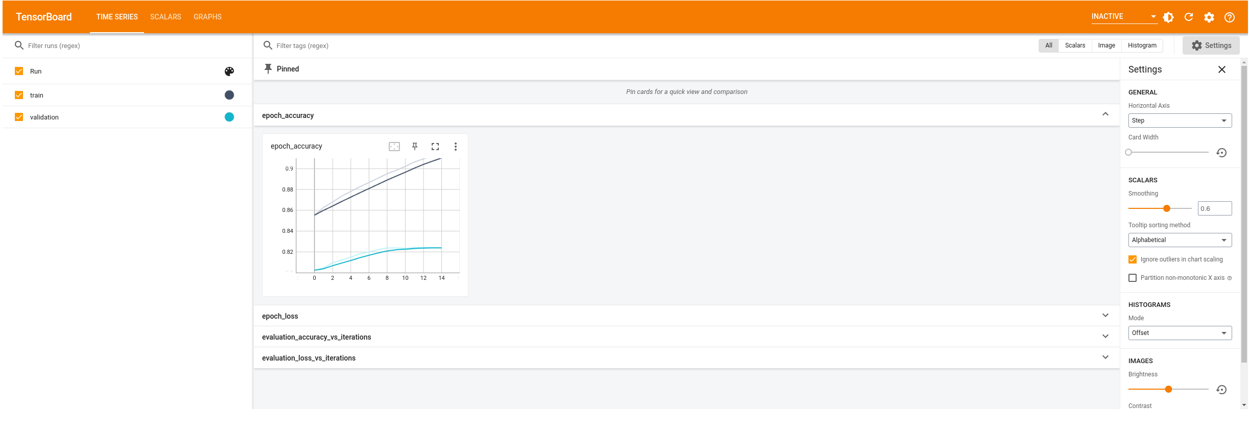
Visualize warm-started training
# docs_infra: no_execute
%reload_ext tensorboard
%tensorboard --logdir logs
Next steps
In this tutorial you learned how to:
- Train a sentiment classification model from scratch on a small vocabulary dataset.
- Update the model architecture and warm start the embedding matrix when the vocabulary size changes.
- Continuously improve model accuracy with expanding datasets
To learn more about embeddings check out the Word2Vec and Transformer model for language understanding tutorials.