 View on TensorFlow.org
|
 Run in Google Colab
|
 View source on GitHub
|
 Download notebook Download notebook
|
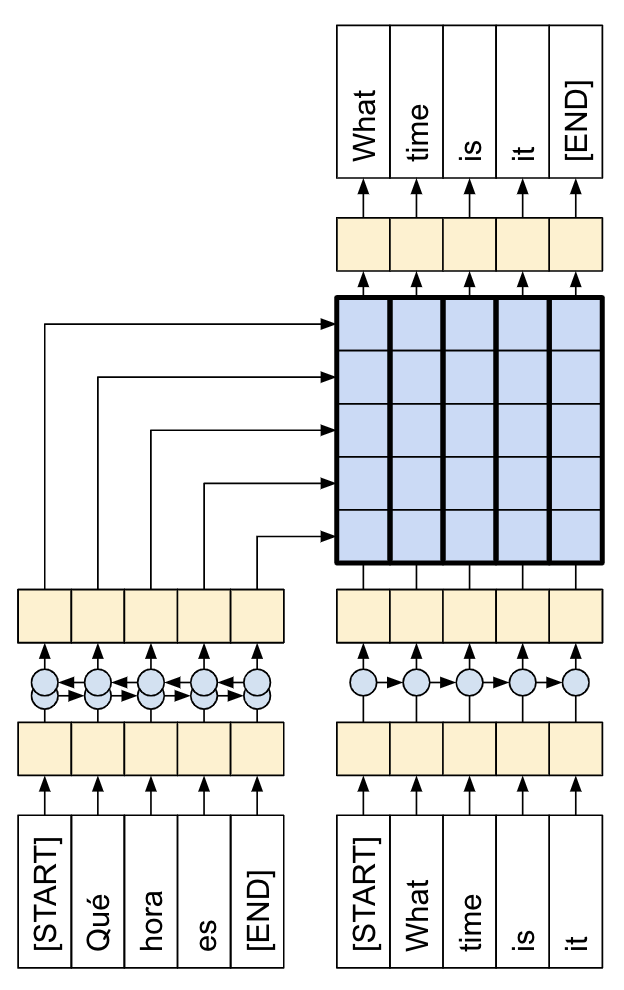
This tutorial demonstrates how to train a sequence-to-sequence (seq2seq) model for Spanish-to-English translation roughly based on Effective Approaches to Attention-based Neural Machine Translation (Luong et al., 2015).
|
| This tutorial: An encoder/decoder connected by attention. |
|---|
While this architecture is somewhat outdated, it is still a very useful project to work through to get a deeper understanding of sequence-to-sequence models and attention mechanisms (before going on to Transformers).
This example assumes some knowledge of TensorFlow fundamentals below the level of a Keras layer:
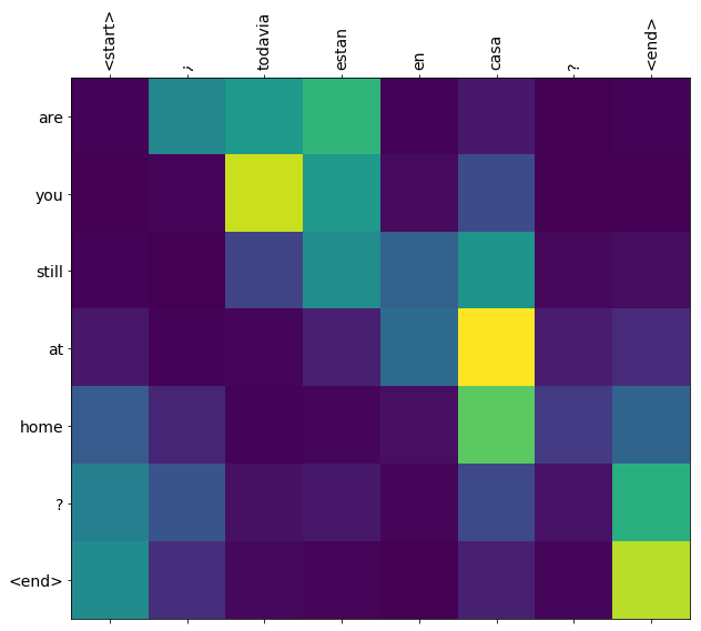
After training the model in this notebook, you will be able to input a Spanish sentence, such as "¿todavia estan en casa?", and return the English translation: "are you still at home?"
The resulting model is exportable as a tf.saved_model, so it can be used in other TensorFlow environments.
The translation quality is reasonable for a toy example, but the generated attention plot is perhaps more interesting. This shows which parts of the input sentence has the model's attention while translating:
Setup
pip install "tensorflow-text>=2.11"pip install einops
import numpy as np

import typing
from typing import Any, Tuple

import einops
import matplotlib.pyplot as plt
import matplotlib.ticker as ticker

import tensorflow as tf
import tensorflow_text as tf_text
This tutorial uses a lot of low level API's where it's easy to get shapes wrong. This class is used to check shapes throughout the tutorial.
class ShapeChecker():
  def __init__(self):
    # Keep a cache of every axis-name seen
    self.shapes = {}

  def __call__(self, tensor, names, broadcast=False):
    if not tf.executing_eagerly():
      return

    parsed = einops.parse_shape(tensor, names)

    for name, new_dim in parsed.items():
      old_dim = self.shapes.get(name, None)

      if (broadcast and new_dim == 1):
        continue

      if old_dim is None:
        # If the axis name is new, add its length to the cache.
        self.shapes[name] = new_dim
        continue

      if new_dim != old_dim:
        raise ValueError(f"Shape mismatch for dimension: '{name}'\n"
                         f"    found: {new_dim}\n"
                         f"    expected: {old_dim}\n")
The data
The tutorial uses a language dataset provided by Anki. This dataset contains language translation pairs in the format:
May I borrow this book? ¿Puedo tomar prestado este libro?
They have a variety of languages available, but this example uses the English-Spanish dataset.
Download and prepare the dataset
For convenience, a copy of this dataset is hosted on Google Cloud, but you can also download your own copy. After downloading the dataset, here are the steps you need to take to prepare the data:
- Add a start and end token to each sentence.
- Clean the sentences by removing special characters.
- Create a word index and reverse word index (dictionaries mapping from word → id and id → word).
- Pad each sentence to a maximum length.
# Download the file
import pathlib

path_to_zip = tf.keras.utils.get_file(
    'spa-eng.zip', origin='http://storage.googleapis.com/download.tensorflow.org/data/spa-eng.zip',
    extract=True)

path_to_file = pathlib.Path(path_to_zip).parent/'spa-eng/spa.txt'
def load_data(path):
  text = path.read_text(encoding='utf-8')

  lines = text.splitlines()
  pairs = [line.split('\t') for line in lines]

  context = np.array([context for target, context in pairs])
  target = np.array([target for target, context in pairs])

  return target, context
target_raw, context_raw = load_data(path_to_file)
print(context_raw[-1])
print(target_raw[-1])
Create a tf.data dataset
From these arrays of strings you can create a tf.data.Dataset of strings that shuffles and batches them efficiently:
BUFFER_SIZE = len(context_raw)
BATCH_SIZE = 64

is_train = np.random.uniform(size=(len(target_raw),)) < 0.8

train_raw = (
    tf.data.Dataset
    .from_tensor_slices((context_raw[is_train], target_raw[is_train]))
    .shuffle(BUFFER_SIZE)
    .batch(BATCH_SIZE))
val_raw = (
    tf.data.Dataset
    .from_tensor_slices((context_raw[~is_train], target_raw[~is_train]))
    .shuffle(BUFFER_SIZE)
    .batch(BATCH_SIZE))
for example_context_strings, example_target_strings in train_raw.take(1):
  print(example_context_strings[:5])
  print()
  print(example_target_strings[:5])
  break
Text preprocessing
One of the goals of this tutorial is to build a model that can be exported as a tf.saved_model. To make that exported model useful it should take tf.string inputs, and return tf.string outputs: All the text processing happens inside the model. Mainly using a layers.TextVectorization layer.
Standardization
The model is dealing with multilingual text with a limited vocabulary. So it will be important to standardize the input text.
The first step is Unicode normalization to split accented characters and replace compatibility characters with their ASCII equivalents.
The tensorflow_text package contains a unicode normalize operation:
example_text = tf.constant('¿Todavía está en casa?')

print(example_text.numpy())
print(tf_text.normalize_utf8(example_text, 'NFKD').numpy())
Unicode normalization will be the first step in the text standardization function:
def tf_lower_and_split_punct(text):
  # Split accented characters.
  text = tf_text.normalize_utf8(text, 'NFKD')
  text = tf.strings.lower(text)
  # Keep space, a to z, and select punctuation.
  text = tf.strings.regex_replace(text, '[^ a-z.?!,¿]', '')
  # Add spaces around punctuation.
  text = tf.strings.regex_replace(text, '[.?!,¿]', r' \0 ')
  # Strip whitespace.
  text = tf.strings.strip(text)

  text = tf.strings.join(['[START]', text, '[END]'], separator=' ')
  return text
print(example_text.numpy().decode())
print(tf_lower_and_split_punct(example_text).numpy().decode())
Text Vectorization
This standardization function will be wrapped up in a tf.keras.layers.TextVectorization layer which will handle the vocabulary extraction and conversion of input text to sequences of tokens.
max_vocab_size = 5000

context_text_processor = tf.keras.layers.TextVectorization(
    standardize=tf_lower_and_split_punct,
    max_tokens=max_vocab_size,
    ragged=True)
The TextVectorization layer and many other Keras preprocessing layers have an adapt method. This method reads one epoch of the training data, and works a lot like Model.fit. This adapt method initializes the layer based on the data. Here it determines the vocabulary:
context_text_processor.adapt(train_raw.map(lambda context, target: context))

# Here are the first 10 words from the vocabulary:
context_text_processor.get_vocabulary()[:10]
That's the Spanish TextVectorization layer, now build and .adapt() the English one:
target_text_processor = tf.keras.layers.TextVectorization(
    standardize=tf_lower_and_split_punct,
    max_tokens=max_vocab_size,
    ragged=True)

target_text_processor.adapt(train_raw.map(lambda context, target: target))
target_text_processor.get_vocabulary()[:10]
Now these layers can convert a batch of strings into a batch of token IDs:
example_tokens = context_text_processor(example_context_strings)
example_tokens[:3, :]
The get_vocabulary method can be used to convert token IDs back to text:
context_vocab = np.array(context_text_processor.get_vocabulary())
tokens = context_vocab[example_tokens[0].numpy()]
' '.join(tokens)
The returned token IDs are zero-padded. This can easily be turned into a mask:
plt.subplot(1, 2, 1)
plt.pcolormesh(example_tokens.to_tensor())
plt.title('Token IDs')

plt.subplot(1, 2, 2)
plt.pcolormesh(example_tokens.to_tensor() != 0)
plt.title('Mask')
Process the dataset
The process_text function below converts the Datasets of strings, into 0-padded tensors of token IDs. It also converts from a (context, target) pair to an ((context, target_in), target_out) pair for training with keras.Model.fit. Keras expects (inputs, labels) pairs, the inputs are the (context, target_in) and the labels are target_out. The difference between target_in and target_out is that they are shifted by one step relative to eachother, so that at each location the label is the next token.
def process_text(context, target):
  context = context_text_processor(context).to_tensor()
  target = target_text_processor(target)
  targ_in = target[:,:-1].to_tensor()
  targ_out = target[:,1:].to_tensor()
  return (context, targ_in), targ_out


train_ds = train_raw.map(process_text, tf.data.AUTOTUNE)
val_ds = val_raw.map(process_text, tf.data.AUTOTUNE)
Here is the first sequence of each, from the first batch:
for (ex_context_tok, ex_tar_in), ex_tar_out in train_ds.take(1):
  print(ex_context_tok[0, :10].numpy())
  print()
  print(ex_tar_in[0, :10].numpy())
  print(ex_tar_out[0, :10].numpy())
The encoder/decoder
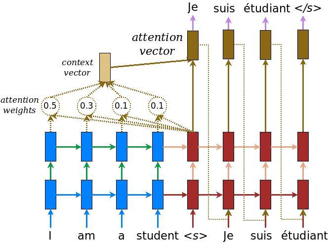
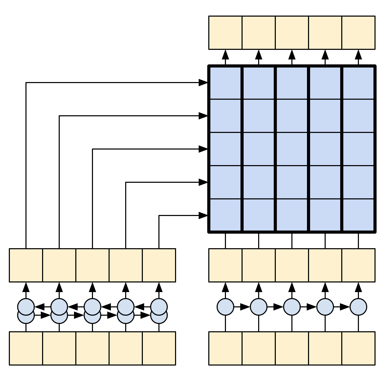
The following diagrams shows an overview of the model. In both the encoder is on the left, the decoder is on the right. At each time-step the decoder's output is combined with the encoder's output, to predict the next word.
The original [left] contains a few extra connections that are intentionally omitted from this tutorial's model [right], as they are generally unnecessary, and difficult to implement. Those missing connections are:
- Feeding the state from the encoder's RNN to the decoder's RNN
- Feeding the attention output back to the RNN's input.
|
|
| The original from Effective Approaches to Attention-based Neural Machine Translation | This tutorial's model |
|---|---|
Before getting into it define constants for the model:
UNITS = 256
The encoder
The goal of the encoder is to process the context sequence into a sequence of vectors that are useful for the decoder as it attempts to predict the next output for each timestep. Since the context sequence is constant, there is no restriction on how information can flow in the encoder, so use a bidirectional-RNN to do the processing:
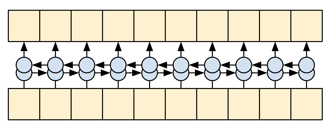
|
| A bidirectional RNN |
|---|
The encoder:
- Takes a list of token IDs (from
context_text_processor). - Looks up an embedding vector for each token (Using a
layers.Embedding). - Processes the embeddings into a new sequence (Using a bidirectional
layers.GRU). - Returns the processed sequence. This will be passed to the attention head.
class Encoder(tf.keras.layers.Layer):
  def __init__(self, text_processor, units):
    super(Encoder, self).__init__()
    self.text_processor = text_processor
    self.vocab_size = text_processor.vocabulary_size()
    self.units = units

    # The embedding layer converts tokens to vectors
    self.embedding = tf.keras.layers.Embedding(self.vocab_size, units,
                                               mask_zero=True)

    # The RNN layer processes those vectors sequentially.
    self.rnn = tf.keras.layers.Bidirectional(
        merge_mode='sum',
        layer=tf.keras.layers.GRU(units,
                            # Return the sequence and state
                            return_sequences=True,
                            recurrent_initializer='glorot_uniform'))

  def call(self, x):
    shape_checker = ShapeChecker()
    shape_checker(x, 'batch s')

    # 2. The embedding layer looks up the embedding vector for each token.
    x = self.embedding(x)
    shape_checker(x, 'batch s units')

    # 3. The GRU processes the sequence of embeddings.
    x = self.rnn(x)
    shape_checker(x, 'batch s units')

    # 4. Returns the new sequence of embeddings.
    return x

  def convert_input(self, texts):
    texts = tf.convert_to_tensor(texts)
    if len(texts.shape) == 0:
      texts = tf.convert_to_tensor(texts)[tf.newaxis]
    context = self.text_processor(texts).to_tensor()
    context = self(context)
    return context
Try it out:
# Encode the input sequence.
encoder = Encoder(context_text_processor, UNITS)
ex_context = encoder(ex_context_tok)

print(f'Context tokens, shape (batch, s): {ex_context_tok.shape}')
print(f'Encoder output, shape (batch, s, units): {ex_context.shape}')
The attention layer
The attention layer lets the decoder access the information extracted by the encoder. It computes a vector from the entire context sequence, and adds that to the decoder's output.
The simplest way you could calculate a single vector from the entire sequence would be to take the average across the sequence (layers.GlobalAveragePooling1D). An attention layer is similar, but calculates a weighted average across the context sequence. Where the weights are calculated from the combination of context and "query" vectors.
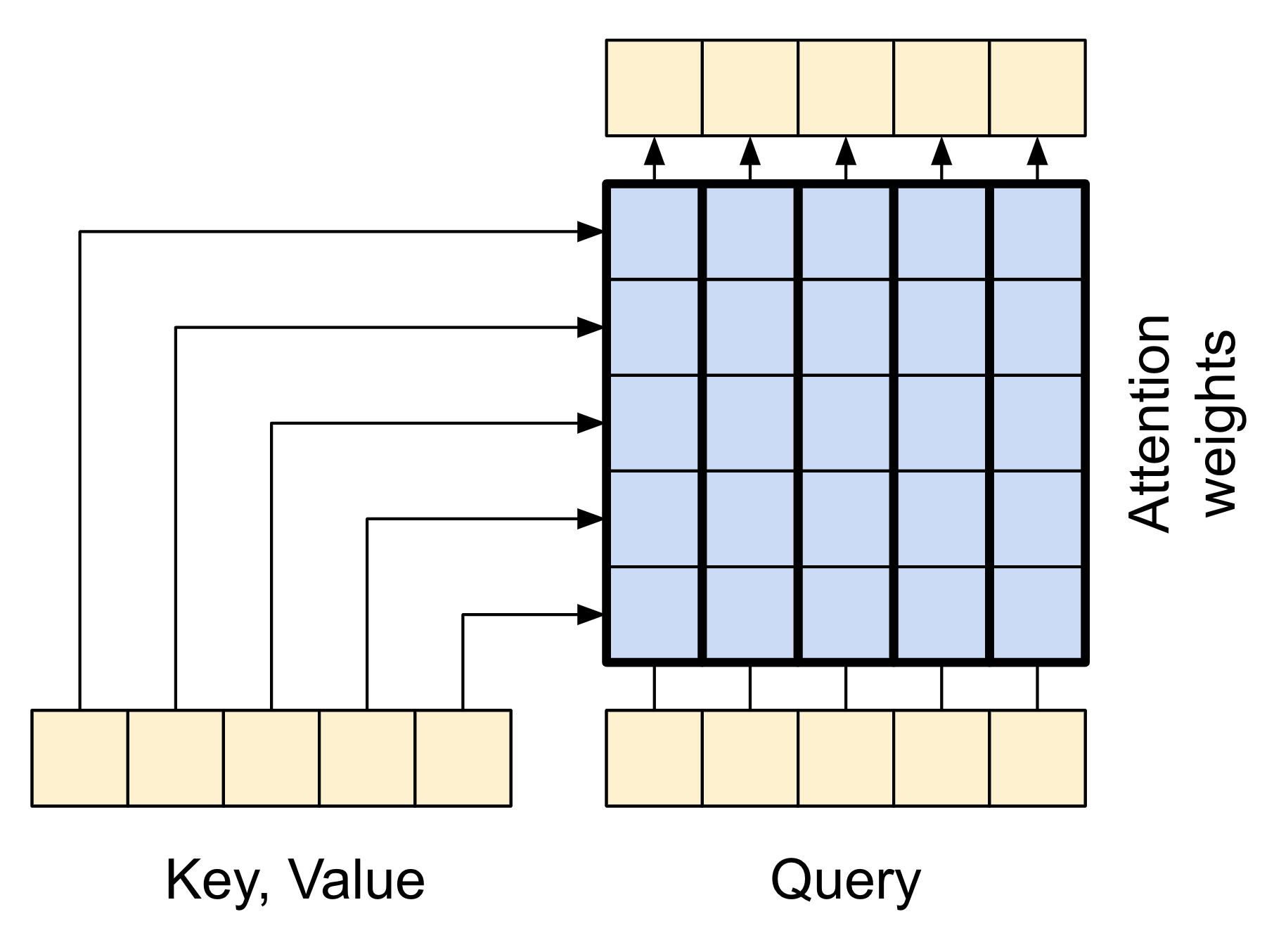
|
| The attention layer |
|---|
class CrossAttention(tf.keras.layers.Layer):
  def __init__(self, units, **kwargs):
    super().__init__()
    self.mha = tf.keras.layers.MultiHeadAttention(key_dim=units, num_heads=1, **kwargs)
    self.layernorm = tf.keras.layers.LayerNormalization()
    self.add = tf.keras.layers.Add()

  def call(self, x, context):
    shape_checker = ShapeChecker()

    shape_checker(x, 'batch t units')
    shape_checker(context, 'batch s units')

    attn_output, attn_scores = self.mha(
        query=x,
        value=context,
        return_attention_scores=True)

    shape_checker(x, 'batch t units')
    shape_checker(attn_scores, 'batch heads t s')

    # Cache the attention scores for plotting later.
    attn_scores = tf.reduce_mean(attn_scores, axis=1)
    shape_checker(attn_scores, 'batch t s')
    self.last_attention_weights = attn_scores

    x = self.add([x, attn_output])
    x = self.layernorm(x)

    return x
attention_layer = CrossAttention(UNITS)

# Attend to the encoded tokens
embed = tf.keras.layers.Embedding(target_text_processor.vocabulary_size(),
                                  output_dim=UNITS, mask_zero=True)
ex_tar_embed = embed(ex_tar_in)

result = attention_layer(ex_tar_embed, ex_context)

print(f'Context sequence, shape (batch, s, units): {ex_context.shape}')
print(f'Target sequence, shape (batch, t, units): {ex_tar_embed.shape}')
print(f'Attention result, shape (batch, t, units): {result.shape}')
print(f'Attention weights, shape (batch, t, s):    {attention_layer.last_attention_weights.shape}')
The attention weights will sum to 1 over the context sequence, at each location in the target sequence.
attention_layer.last_attention_weights[0].numpy().sum(axis=-1)
Here are the attention weights across the context sequences at t=0:
attention_weights = attention_layer.last_attention_weights
mask=(ex_context_tok != 0).numpy()

plt.subplot(1, 2, 1)
plt.pcolormesh(mask*attention_weights[:, 0, :])
plt.title('Attention weights')

plt.subplot(1, 2, 2)
plt.pcolormesh(mask)
plt.title('Mask');
Because of the small-random initialization the attention weights are initially all close to 1/(sequence_length). The model will learn to make these less uniform as training progresses.
The decoder
The decoder's job is to generate predictions for the next token at each location in the target sequence.
- It looks up embeddings for each token in the target sequence.
- It uses an RNN to process the target sequence, and keep track of what it has generated so far.
- It uses RNN output as the "query" to the attention layer, when attending to the encoder's output.
- At each location in the output it predicts the next token.
When training, the model predicts the next word at each location. So it's important that the information only flows in one direction through the model. The decoder uses a unidirectional (not bidirectional) RNN to process the target sequence.
When running inference with this model it produces one word at a time, and those are fed back into the model.
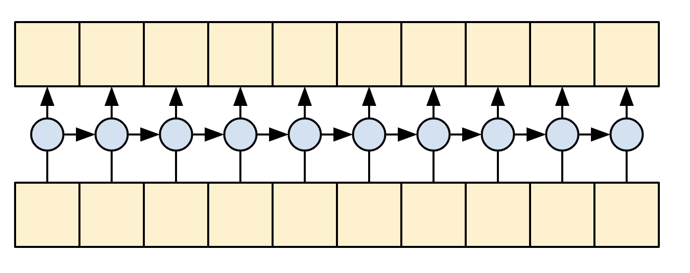
|
| A unidirectional RNN |
|---|
Here is the Decoder class' initializer. The initializer creates all the necessary layers.
class Decoder(tf.keras.layers.Layer):
  @classmethod
  def add_method(cls, fun):
    setattr(cls, fun.__name__, fun)
    return fun

  def __init__(self, text_processor, units):
    super(Decoder, self).__init__()
    self.text_processor = text_processor
    self.vocab_size = text_processor.vocabulary_size()
    self.word_to_id = tf.keras.layers.StringLookup(
        vocabulary=text_processor.get_vocabulary(),
        mask_token='', oov_token='[UNK]')
    self.id_to_word = tf.keras.layers.StringLookup(
        vocabulary=text_processor.get_vocabulary(),
        mask_token='', oov_token='[UNK]',
        invert=True)
    self.start_token = self.word_to_id('[START]')
    self.end_token = self.word_to_id('[END]')

    self.units = units


    # 1. The embedding layer converts token IDs to vectors
    self.embedding = tf.keras.layers.Embedding(self.vocab_size,
                                               units, mask_zero=True)

    # 2. The RNN keeps track of what's been generated so far.
    self.rnn = tf.keras.layers.GRU(units,
                                   return_sequences=True,
                                   return_state=True,
                                   recurrent_initializer='glorot_uniform')

    # 3. The RNN output will be the query for the attention layer.
    self.attention = CrossAttention(units)

    # 4. This fully connected layer produces the logits for each
    # output token.
    self.output_layer = tf.keras.layers.Dense(self.vocab_size)
Training
Next, the call method, takes 3 arguments:
inputs- acontext, xpair where:context- is the context from the encoder's output.x- is the target sequence input.
state- Optional, the previousstateoutput from the decoder (the internal state of the decoder's RNN). Pass the state from a previous run to continue generating text where you left off.return_state- [Default: False] - Set this toTrueto return the RNN state.
@Decoder.add_method
def call(self,
         context, x,
         state=None,
         return_state=False):
  shape_checker = ShapeChecker()
  shape_checker(x, 'batch t')
  shape_checker(context, 'batch s units')

  # 1. Lookup the embeddings
  x = self.embedding(x)
  shape_checker(x, 'batch t units')

  # 2. Process the target sequence.
  x, state = self.rnn(x, initial_state=state)
  shape_checker(x, 'batch t units')

  # 3. Use the RNN output as the query for the attention over the context.
  x = self.attention(x, context)
  self.last_attention_weights = self.attention.last_attention_weights
  shape_checker(x, 'batch t units')
  shape_checker(self.last_attention_weights, 'batch t s')

  # Step 4. Generate logit predictions for the next token.
  logits = self.output_layer(x)
  shape_checker(logits, 'batch t target_vocab_size')

  if return_state:
    return logits, state
  else:
    return logits
That will be sufficient for training. Create an instance of the decoder to test out:
decoder = Decoder(target_text_processor, UNITS)
In training you'll use the decoder like this:
Given the context and target tokens, for each target token it predicts the next target token.
logits = decoder(ex_context, ex_tar_in)

print(f'encoder output shape: (batch, s, units) {ex_context.shape}')
print(f'input target tokens shape: (batch, t) {ex_tar_in.shape}')
print(f'logits shape shape: (batch, target_vocabulary_size) {logits.shape}')
Inference
To use it for inference you'll need a couple more methods:
@Decoder.add_method
def get_initial_state(self, context):
  batch_size = tf.shape(context)[0]
  start_tokens = tf.fill([batch_size, 1], self.start_token)
  done = tf.zeros([batch_size, 1], dtype=tf.bool)
  embedded = self.embedding(start_tokens)
  return start_tokens, done, self.rnn.get_initial_state(embedded)[0]
@Decoder.add_method
def tokens_to_text(self, tokens):
  words = self.id_to_word(tokens)
  result = tf.strings.reduce_join(words, axis=-1, separator=' ')
  result = tf.strings.regex_replace(result, '^ *\[START\] *', '')
  result = tf.strings.regex_replace(result, ' *\[END\] *$', '')
  return result
@Decoder.add_method
def get_next_token(self, context, next_token, done, state, temperature = 0.0):
  logits, state = self(
    context, next_token,
    state = state,
    return_state=True)

  if temperature == 0.0:
    next_token = tf.argmax(logits, axis=-1)
  else:
    logits = logits[:, -1, :]/temperature
    next_token = tf.random.categorical(logits, num_samples=1)

  # If a sequence produces an `end_token`, set it `done`
  done = done | (next_token == self.end_token)
  # Once a sequence is done it only produces 0-padding.
  next_token = tf.where(done, tf.constant(0, dtype=tf.int64), next_token)

  return next_token, done, state
With those extra functions, you can write a generation loop:
# Setup the loop variables.
next_token, done, state = decoder.get_initial_state(ex_context)
tokens = []

for n in range(10):
  # Run one step.
  next_token, done, state = decoder.get_next_token(
      ex_context, next_token, done, state, temperature=1.0)
  # Add the token to the output.
  tokens.append(next_token)

# Stack all the tokens together.
tokens = tf.concat(tokens, axis=-1) # (batch, t)

# Convert the tokens back to a a string
result = decoder.tokens_to_text(tokens)
result[:3].numpy()
Since the model's untrained, it outputs items from the vocabulary almost uniformly at random.
The model
Now that you have all the model components, combine them to build the model for training:
class Translator(tf.keras.Model):
  @classmethod
  def add_method(cls, fun):
    setattr(cls, fun.__name__, fun)
    return fun

  def __init__(self, units,
               context_text_processor,
               target_text_processor):
    super().__init__()
    # Build the encoder and decoder
    encoder = Encoder(context_text_processor, units)
    decoder = Decoder(target_text_processor, units)

    self.encoder = encoder
    self.decoder = decoder

  def call(self, inputs):
    context, x = inputs
    context = self.encoder(context)
    logits = self.decoder(context, x)

    #TODO(b/250038731): remove this
    try:
      # Delete the keras mask, so keras doesn't scale the loss+accuracy.
      del logits._keras_mask
    except AttributeError:
      pass

    return logits
During training the model will be used like this:
model = Translator(UNITS, context_text_processor, target_text_processor)

logits = model((ex_context_tok, ex_tar_in))

print(f'Context tokens, shape: (batch, s, units) {ex_context_tok.shape}')
print(f'Target tokens, shape: (batch, t) {ex_tar_in.shape}')
print(f'logits, shape: (batch, t, target_vocabulary_size) {logits.shape}')
Train
For training, you'll want to implement your own masked loss and accuracy functions:
def masked_loss(y_true, y_pred):
    # Calculate the loss for each item in the batch.
    loss_fn = tf.keras.losses.SparseCategoricalCrossentropy(
        from_logits=True, reduction='none')
    loss = loss_fn(y_true, y_pred)

    # Mask off the losses on padding.
    mask = tf.cast(y_true != 0, loss.dtype)
    loss *= mask

    # Return the total.
    return tf.reduce_sum(loss)/tf.reduce_sum(mask)
def masked_acc(y_true, y_pred):
    # Calculate the loss for each item in the batch.
    y_pred = tf.argmax(y_pred, axis=-1)
    y_pred = tf.cast(y_pred, y_true.dtype)

    match = tf.cast(y_true == y_pred, tf.float32)
    mask = tf.cast(y_true != 0, tf.float32)

    return tf.reduce_sum(match)/tf.reduce_sum(mask)
Configure the model for training:
model.compile(optimizer='adam',
              loss=masked_loss,
              metrics=[masked_acc, masked_loss])
The model is randomly initialized, and should give roughly uniform output probabilities. So it's easy to predict what the initial values of the metrics should be:
vocab_size = 1.0 * target_text_processor.vocabulary_size()

{"expected_loss": tf.math.log(vocab_size).numpy(),
 "expected_acc": 1/vocab_size}
That should roughly match the values returned by running a few steps of evaluation:
model.evaluate(val_ds, steps=20, return_dict=True)
history = model.fit(
    train_ds.repeat(),
    epochs=100,
    steps_per_epoch = 100,
    validation_data=val_ds,
    validation_steps = 20,
    callbacks=[
        tf.keras.callbacks.EarlyStopping(patience=3)])
plt.plot(history.history['loss'], label='loss')
plt.plot(history.history['val_loss'], label='val_loss')
plt.ylim([0, max(plt.ylim())])
plt.xlabel('Epoch #')
plt.ylabel('CE/token')
plt.legend()
plt.plot(history.history['masked_acc'], label='accuracy')
plt.plot(history.history['val_masked_acc'], label='val_accuracy')
plt.ylim([0, max(plt.ylim())])
plt.xlabel('Epoch #')
plt.ylabel('CE/token')
plt.legend()
Translate
Now that the model is trained, implement a function to execute the full text => text translation. This code is basically identical to the inference example in the decoder section, but this also captures the attention weights.
@Translator.add_method
def translate(self,
              texts, *,
              max_length=50,
              temperature=0.0):
  # Process the input texts
  context = self.encoder.convert_input(texts)
  batch_size = tf.shape(texts)[0]

  # Setup the loop inputs
  tokens = []
  attention_weights = []
  next_token, done, state = self.decoder.get_initial_state(context)

  for _ in range(max_length):
    # Generate the next token
    next_token, done, state = self.decoder.get_next_token(
        context, next_token, done,  state, temperature)

    # Collect the generated tokens
    tokens.append(next_token)
    attention_weights.append(self.decoder.last_attention_weights)

    if tf.executing_eagerly() and tf.reduce_all(done):
      break

  # Stack the lists of tokens and attention weights.
  tokens = tf.concat(tokens, axis=-1)   # t*[(batch 1)] -> (batch, t)
  self.last_attention_weights = tf.concat(attention_weights, axis=1)  # t*[(batch 1 s)] -> (batch, t s)

  result = self.decoder.tokens_to_text(tokens)
  return result
Here are the two helper methods, used above, to convert tokens to text, and to get the next token:
result = model.translate(['¿Todavía está en casa?']) # Are you still home
result[0].numpy().decode()
Use that to generate the attention plot:
@Translator.add_method
def plot_attention(self, text, **kwargs):
  assert isinstance(text, str)
  output = self.translate([text], **kwargs)
  output = output[0].numpy().decode()

  attention = self.last_attention_weights[0]

  context = tf_lower_and_split_punct(text)
  context = context.numpy().decode().split()

  output = tf_lower_and_split_punct(output)
  output = output.numpy().decode().split()[1:]

  fig = plt.figure(figsize=(10, 10))
  ax = fig.add_subplot(1, 1, 1)

  ax.matshow(attention, cmap='viridis', vmin=0.0)

  fontdict = {'fontsize': 14}

  ax.set_xticklabels([''] + context, fontdict=fontdict, rotation=90)
  ax.set_yticklabels([''] + output, fontdict=fontdict)

  ax.xaxis.set_major_locator(ticker.MultipleLocator(1))
  ax.yaxis.set_major_locator(ticker.MultipleLocator(1))

  ax.set_xlabel('Input text')
  ax.set_ylabel('Output text')
model.plot_attention('¿Todavía está en casa?') # Are you still home
Translate a few more sentences and plot them:
%%time
# This is my life.
model.plot_attention('Esta es mi vida.')
%%time
 # Try to find out.'
model.plot_attention('Tratar de descubrir.')
The short sentences often work well, but if the input is too long the model literally loses focus and stops providing reasonable predictions. There are two main reasons for this:
- The model was trained with teacher-forcing feeding the correct token at each step, regardless of the model's predictions. The model could be made more robust if it were sometimes fed its own predictions.
- The model only has access to its previous output through the RNN state. If the RNN state looses track of where it was in the context sequence there's no way for the model to recover. Transformers improve on this by letting the decoder look at what it has output so far.
The raw data is sorted by length, so try translating the longest sequence:
long_text = context_raw[-1]

import textwrap
print('Expected output:\n', '\n'.join(textwrap.wrap(target_raw[-1])))
model.plot_attention(long_text)
The translate function works on batches, so if you have multiple texts to translate you can pass them all at once, which is much more efficient than translating them one at a time:
inputs = [
    'Hace mucho frio aqui.', # "It's really cold here."
    'Esta es mi vida.', # "This is my life."
    'Su cuarto es un desastre.' # "His room is a mess"
]
%%time
for t in inputs:
  print(model.translate([t])[0].numpy().decode())

print()
%%time
result = model.translate(inputs)

print(result[0].numpy().decode())
print(result[1].numpy().decode())
print(result[2].numpy().decode())
print()
So overall this text generation function mostly gets the job done, but so you've only used it here in python with eager execution. Let's try to export it next:
Export
If you want to export this model you'll need to wrap the translate method in a tf.function. That implementation will get the job done:
class Export(tf.Module):
  def __init__(self, model):
    self.model = model

  @tf.function(input_signature=[tf.TensorSpec(dtype=tf.string, shape=[None])])
  def translate(self, inputs):
    return self.model.translate(inputs)
export = Export(model)
Run the tf.function once to compile it:
%%time
_ = export.translate(tf.constant(inputs))
%%time
result = export.translate(tf.constant(inputs))

print(result[0].numpy().decode())
print(result[1].numpy().decode())
print(result[2].numpy().decode())
print()
Now that the function has been traced it can be exported using saved_model.save:
%%time
tf.saved_model.save(export, 'translator',
                    signatures={'serving_default': export.translate})
%%time
reloaded = tf.saved_model.load('translator')
_ = reloaded.translate(tf.constant(inputs)) #warmup
%%time
result = reloaded.translate(tf.constant(inputs))

print(result[0].numpy().decode())
print(result[1].numpy().decode())
print(result[2].numpy().decode())
print()
[Optional] Use a dynamic loop
It's worth noting that this initial implementation is not optimal. It uses a python loop:
for _ in range(max_length):
  ...
  if tf.executing_eagerly() and tf.reduce_all(done):
    break
The python loop is relatively simple but when tf.function converts this to a graph, it statically unrolls that loop. Unrolling the loop has two disadvantages:
- It makes
max_lengthcopies of the loop body. So the generated graphs take longer to build, save and load. - You have to choose a fixed value for the
max_length. - You can't
breakfrom a statically unrolled loop. Thetf.functionversion will run the fullmax_lengthiterations on every call. That's why thebreakonly works with eager execution. This is still marginally faster than eager execution, but not as fast as it could be.
To fix these shortcomings, the translate_dynamic method, below, uses a tensorflow loop:
for t in tf.range(max_length):
  ...
  if tf.reduce_all(done):
      break
It looks like a python loop, but when you use a tensor as the input to a for loop (or the condition of a while loop) tf.function converts it to a dynamic loop using operations like tf.while_loop.
There's no need for a max_length here it's just in case the model gets stuck generating a loop like: the united states of the united states of the united states....
On the down side, to accumulate tokens from this dynamic loop you can't just append them to a python list, you need to use a tf.TensorArray:
tokens = tf.TensorArray(tf.int64, size=1, dynamic_size=True)
...
for t in tf.range(max_length):
    ...
    tokens = tokens.write(t, next_token) # next_token shape is (batch, 1)
  ...
  tokens = tokens.stack()
  tokens = einops.rearrange(tokens, 't batch 1 -> batch t')
This version of the code can be quite a bit more efficient:
@Translator.add_method
def translate(self,
              texts,
              *,
              max_length=500,
              temperature=tf.constant(0.0)):
  shape_checker = ShapeChecker()
  context = self.encoder.convert_input(texts)
  batch_size = tf.shape(context)[0]
  shape_checker(context, 'batch s units')

  next_token, done, state = self.decoder.get_initial_state(context)

  # initialize the accumulator
  tokens = tf.TensorArray(tf.int64, size=1, dynamic_size=True)

  for t in tf.range(max_length):
    # Generate the next token
    next_token, done, state = self.decoder.get_next_token(
        context, next_token, done, state, temperature)
    shape_checker(next_token, 'batch t1')

    # Collect the generated tokens
    tokens = tokens.write(t, next_token)

    # if all the sequences are done, break
    if tf.reduce_all(done):
      break

  # Convert the list of generated token ids to a list of strings.
  tokens = tokens.stack()
  shape_checker(tokens, 't batch t1')
  tokens = einops.rearrange(tokens, 't batch 1 -> batch t')
  shape_checker(tokens, 'batch t')

  text = self.decoder.tokens_to_text(tokens)
  shape_checker(text, 'batch')

  return text
With eager execution this implementation performs on par with the original:
%%time
result = model.translate(inputs)

print(result[0].numpy().decode())
print(result[1].numpy().decode())
print(result[2].numpy().decode())
print()
But when you wrap it in a tf.function you'll notice two differences.
class Export(tf.Module):
  def __init__(self, model):
    self.model = model

  @tf.function(input_signature=[tf.TensorSpec(dtype=tf.string, shape=[None])])
  def translate(self, inputs):
    return self.model.translate(inputs)
export = Export(model)
First, it's much quicker to trace, since it only creates one copy of the loop body:
%%time
_ = export.translate(inputs)
The tf.function is much faster than running with eager execution, and on small inputs it's often several times faster than the unrolled version, because it can break out of the loop.
%%time
result = export.translate(inputs)

print(result[0].numpy().decode())
print(result[1].numpy().decode())
print(result[2].numpy().decode())
print()
So save this version as well:
%%time
tf.saved_model.save(export, 'dynamic_translator',
                    signatures={'serving_default': export.translate})
%%time
reloaded = tf.saved_model.load('dynamic_translator')
_ = reloaded.translate(tf.constant(inputs)) #warmup
%%time
result = reloaded.translate(tf.constant(inputs))

print(result[0].numpy().decode())
print(result[1].numpy().decode())
print(result[2].numpy().decode())
print()
Next steps
- Download a different dataset to experiment with translations, for example, English to German, or English to French.
- Experiment with training on a larger dataset, or using more epochs.
- Try the transformer tutorial which implements a similar translation task but uses transformer layers instead of RNNs. This version also uses a
text.BertTokenizerto implement word-piece tokenization. - Visit the
tensorflow_addons.seq2seqtutorial, which demonstrates a higher-level functionality for implementing this sort of sequence-to-sequence model, such asseq2seq.BeamSearchDecoder.
