Uplifting with Decision Forests

Welcome to the Uplifting Tutorial for TensorFlow Decision Forests (TF-DF). In this tutorial, you will learn what uplifting is, why it is so important, and how to do it in TF-DF.

This tutorial assumes you are familiar with the fundaments of TF-DF, in particular the installation procedure. The beginner tutorial is a great place to start learning about TF-DF.

In this colab, you will:

• Learn what an uplift modeling is.
• Train a Uplift Random Forest model on the Hillstrom Email Marketing dataset.
• Evaluate the quality of this model.

Installing TensorFlow Decision Forests

Install TF-DF by running the following cell.

Wurlitzer is needed to display the detailed training logs in Colabs (when using verbose=2 in the model constructor).

Tensorflow Datasets is needed download the dataset used in this tutorial.

pip install tensorflow_decision_forests wurlitzer tensorflow-datasets

Importing libraries

import tensorflow_decision_forests as tfdf

import os
import numpy as np
import pandas as pd
import tensorflow as tf
import math
import matplotlib.pyplot as plt

2025-02-26 12:05:36.978454: E external/local_xla/xla/stream_executor/cuda/cuda_fft.cc:477] Unable to register cuFFT factory: Attempting to register factory for plugin cuFFT when one has already been registered
WARNING: All log messages before absl::InitializeLog() is called are written to STDERR
E0000 00:00:1740571537.000097    9083 cuda_dnn.cc:8310] Unable to register cuDNN factory: Attempting to register factory for plugin cuDNN when one has already been registered
E0000 00:00:1740571537.006625    9083 cuda_blas.cc:1418] Unable to register cuBLAS factory: Attempting to register factory for plugin cuBLAS when one has already been registered

The hidden code cell limits the output height in colab.

Toggle code

from IPython.core.magic import register_line_magic
from IPython.display import Javascript
from IPython.display import display as ipy_display

# Some of the model training logs can cover the full
# screen if not compressed to a smaller viewport.
# This magic allows setting a max height for a cell.
@register_line_magic
def set_cell_height(size):
  ipy_display(
      Javascript("google.colab.output.setIframeHeight(0, true, {maxHeight: " +
                 str(size) + "})"))

# Check the version of TensorFlow Decision Forests
print("Found TensorFlow Decision Forests v" + tfdf.__version__)

Found TensorFlow Decision Forests v1.11.0

What is uplift modeling?

Uplift modeling is a statistical modeling technique to predict the incremental impact of an action on a subject. The action is often referred to as a treatment that may or may not be applied.

Uplift modeling is often used in targeted marketing campaigns to predict the increase in the likelihood of a person making a purchase (or any other desired action) based on the marketing exposition they receive.

For example, uplift modeling can predict the effect of an email. The effect is defined as the conditional probability \begin{align} \text{effect}(\text{email}) = &\Pr(\text{outcome}=\text{purchase}\ \vert\ \text{treatment}=\text{with email})\ &- \Pr(\text{outcome}=\text{purchase} \ \vert\ \text{treatment}=\text{no email}), \end{align} where \(\Pr(\text{outcome}=\text{purchase}\ \vert\ ...)\) is the probability of purchase depending on the receiving or not an email.

Compare this to a classification model: With a classification model, one can predict the probability of a purchase. However, customers with a high probability are likely to spend money in the store regardless of whether or not they received an email.

Similarly, one can use numerical uplifting to predict the numerical increase in spend when receiving an email. In comparison, a regression model can only increase the expected spend, which is a less useful metric in many cases.

Defining uplift models in TF-DF

TF-DF expects uplifting datasets to be presented in a "flat" format. A dataset of customers might look like this

treatment	outcome	feature_1	feature_2
0	1	0.1	blue
0	0	0.2	blue
1	1	0.3	blue
1	1	0.4	blue

The treatment is a binary variable indicating whether or not the example has received treatment. In the above example, the treatment indicates if the customer has received an email or not. The outcome (label) indicates the status of the example after receiving the treatment (or not). TF-DF supports categorical outcomes for categorical uplifting and numerical outcomes for numerical uplifting.

Note: Uplifting is also frequently used in medical contexts. Here the treatment can be a medical treatment (e.g. administering a vaccine), the label can be an indicator of quality of life (e.g. whether the patient got sick). This also explains the nomenclature of uplift modeling.

Training an uplifting model

In this example, we will use the Hillstrom Email Marketing dataset.

This dataset contains 64,000 customers who last purchased within twelve months. The customers were involved in an e-mail test:

• 1/3 were randomly chosen to receive an e-mail campaign featuring Mens merchandise.
• 1/3 were randomly chosen to receive an e-mail campaign featuring Womens merchandise.
• 1/3 were randomly chosen to not receive an e-mail campaign.

During a period of two weeks following the e-mail campaign, results were tracked. The task is to tell if the Mens or Womens e-mail campaign was successful.

Read more about dataset in its documentation. This tutorial uses the dataset as curated by TensorFlow Datasets.

# Load the dataset
import tensorflow_datasets as tfds
raw_train, raw_test = tfds.load('hillstrom', split=['train[:80%]', 'train[20%:]'])

# Display the first 10 examples of the test fold.
pd.DataFrame(list(raw_test.batch(10).take(1))[0])

I0000 00:00:1740571542.697544    9083 gpu_device.cc:2022] Created device /job:localhost/replica:0/task:0/device:GPU:0 with 13638 MB memory:  -> device: 0, name: Tesla T4, pci bus id: 0000:00:05.0, compute capability: 7.5
I0000 00:00:1740571542.699822    9083 gpu_device.cc:2022] Created device /job:localhost/replica:0/task:0/device:GPU:1 with 13756 MB memory:  -> device: 1, name: Tesla T4, pci bus id: 0000:00:06.0, compute capability: 7.5
I0000 00:00:1740571542.701960    9083 gpu_device.cc:2022] Created device /job:localhost/replica:0/task:0/device:GPU:2 with 13756 MB memory:  -> device: 2, name: Tesla T4, pci bus id: 0000:00:07.0, compute capability: 7.5
I0000 00:00:1740571542.703996    9083 gpu_device.cc:2022] Created device /job:localhost/replica:0/task:0/device:GPU:3 with 13756 MB memory:  -> device: 3, name: Tesla T4, pci bus id: 0000:00:08.0, compute capability: 7.5
2025-02-26 12:05:43.599785: W tensorflow/core/kernels/data/cache_dataset_ops.cc:914] The calling iterator did not fully read the dataset being cached. In order to avoid unexpected truncation of the dataset, the partially cached contents of the dataset  will be discarded. This can happen if you have an input pipeline similar to `dataset.cache().take(k).repeat()`. You should use `dataset.take(k).cache().repeat()` instead.

Dataset preprocessing

Since TF-DF currently only supports binary treatments, combine the "Men's Email" and the "Women's Email" campaign. This tutorial uses the binary variable conversion as outcome. This means that the problem is a Categorical Uplifting problem. If we were using the numerical variable spend, the problem would be a Numerical Uplifting problem.

def prepare_dataset(example):
  # Use a binary treatment class.
  example['treatment'] = 1 if example['segment'] == b'Mens E-Mail' or example['segment'] == b'Womens E-Mail' else 0
  outcome = example['conversion']
  # Restrict the dataset to the input features.
  input_features = ['channel', 'history', 'mens', 'womens', 'newbie', 'recency', 'zip_code', 'treatment']
  example = {feature: example[feature] for feature in input_features}
  return example, outcome

train_ds = raw_train.map(prepare_dataset).batch(100)
test_ds = raw_test.map(prepare_dataset).batch(100)

Model training

Finally, train and evaluate the model as usual. Note that TF-DF only supports Random Forest models for uplifting.

%set_cell_height 300

# Configure the model and its hyper-parameters.
model = tfdf.keras.RandomForestModel(
    verbose=2,
    task=tfdf.keras.Task.CATEGORICAL_UPLIFT,
    uplift_treatment='treatment'
)

# Train the model.
model.fit(train_ds)

<IPython.core.display.Javascript object>
Warning: The `num_threads` constructor argument is not set and the number of CPU is os.cpu_count()=32 > 32. Setting num_threads to 32. Set num_threads manually to use more than 32 cpus.
WARNING:absl:The `num_threads` constructor argument is not set and the number of CPU is os.cpu_count()=32 > 32. Setting num_threads to 32. Set num_threads manually to use more than 32 cpus.
Use /tmpfs/tmp/tmphsli6pat as temporary training directory
Reading training dataset...
Training tensor examples:
Features: {'channel': <tf.Tensor 'data:0' shape=(None,) dtype=string>, 'history': <tf.Tensor 'data_1:0' shape=(None,) dtype=float32>, 'mens': <tf.Tensor 'data_2:0' shape=(None,) dtype=int64>, 'womens': <tf.Tensor 'data_3:0' shape=(None,) dtype=int64>, 'newbie': <tf.Tensor 'data_4:0' shape=(None,) dtype=int64>, 'recency': <tf.Tensor 'data_5:0' shape=(None,) dtype=int64>, 'zip_code': <tf.Tensor 'data_6:0' shape=(None,) dtype=string>, 'treatment': <tf.Tensor 'data_7:0' shape=(None,) dtype=int32>}
Label: Tensor("data_8:0", shape=(None,), dtype=int64)
Weights: None
Normalized tensor features:
 {'channel': SemanticTensor(semantic=<Semantic.CATEGORICAL: 2>, tensor=<tf.Tensor 'data:0' shape=(None,) dtype=string>), 'history': SemanticTensor(semantic=<Semantic.NUMERICAL: 1>, tensor=<tf.Tensor 'data_1:0' shape=(None,) dtype=float32>), 'mens': SemanticTensor(semantic=<Semantic.NUMERICAL: 1>, tensor=<tf.Tensor 'Cast:0' shape=(None,) dtype=float32>), 'womens': SemanticTensor(semantic=<Semantic.NUMERICAL: 1>, tensor=<tf.Tensor 'Cast_1:0' shape=(None,) dtype=float32>), 'newbie': SemanticTensor(semantic=<Semantic.NUMERICAL: 1>, tensor=<tf.Tensor 'Cast_2:0' shape=(None,) dtype=float32>), 'recency': SemanticTensor(semantic=<Semantic.NUMERICAL: 1>, tensor=<tf.Tensor 'Cast_3:0' shape=(None,) dtype=float32>), 'zip_code': SemanticTensor(semantic=<Semantic.CATEGORICAL: 2>, tensor=<tf.Tensor 'data_6:0' shape=(None,) dtype=string>)}
Training dataset read in 0:00:05.088312. Found 51200 examples.
Training model...
Standard output detected as not visible to the user e.g. running in a notebook. Creating a training log redirection. If training gets stuck, try calling tfdf.keras.set_training_logs_redirection(False).
Model trained in 0:00:02.392275
Compiling model...
Model compiled.
<tf_keras.src.callbacks.History at 0x7fad780f9e50>

Evaluating Uplift models.

Metrics for Uplift models

The two most important metrics for evaluating upift models are the AUUC (Area Under the Uplift Curve) metric and the Qini (Area Under the Qini Curve) metric. This is similar to the use of AUC and accuracy for classification problems. For both metrics, the larger they are, the better.

Both AUUC and Qini are not normalized metrics. This means that the best possible value of the metric can vary from dataset to dataset. This is different from, for example, the AUC matric that always varies between 0 and 1.

A formal definition of AUUC is below. For more information about these metrics, see Guelman and Betlei et al.

Model Self-Evaluation

TF-DF Random Forest models perform self-evaluation on the out-of-bag examples of the training dataset. For uplift models, they expose the AUUC and the Qini metric. You can directly retrieve the two metrics on the training dataset through the inspector

Later, we are going to recompute the AUUC metric "manually" on the test dataset. Note that two metrics are not expected to be exactly equal (out-of-bag on train vs test) since the AUUC is not a normalized metric.

# The self-evaluation is available through the model inspector
insp = model.make_inspector()
insp.evaluation()

Evaluation(num_examples=51200, accuracy=None, loss=None, rmse=None, ndcg=None, aucs=None, auuc=0.0022032308892709586, qini=-0.00017325819500263418)

Manually computing the AUUC

In this section, we manually compute the AUUC and plot the uplift curves.

The next few paragraphs explain the AUUC metric in more detail and may be skipped.

Computing the AUUC

Suppose you have a labeled dataset with \(|T|\) examples with treatment and \(|C|\) examples without treatment, called control examples. For each example, the uplift model \(f\) produces the conditional probability that a treatment on the example will yield a positive outcome.

Suppose a decision-maker needs to decide which clients to send an email using an uplift model \(f\). The model produces a (conditional) probability that the email will result in a conversion. The decision-maker might therefore just pick the number \(k\) of emails to send and send those \(k\) emails to the clients with the highest probability.

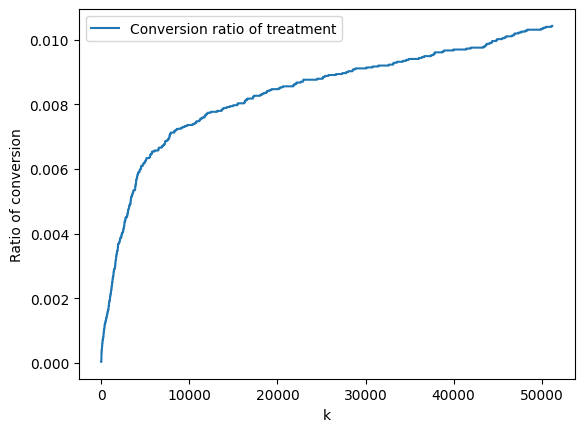
Using a labeled test dataset, it is possible to study the impact of \(k\) on the success of the campaign. First, we are interested in the ratio \(\frac{|C \cap T|}{|T|}\) of clients that received an email that converted versus total number of clients that received an email. Here \(C\) is the set of clients that received an email and converted and \(T\) is the total number of clients that received an email. We plot this ratio against \(k\).

Ideally, we like to have this curve increase steeply. This would mean that the model prioritizes sending email to those clients that will generate a conversion when receiving an email.

# Compute all predictions on the test dataset
predictions = model.predict(test_ds).flatten()
# Extract outcomes and treatments
outcomes = np.concatenate([outcome.numpy() for _, outcome in test_ds])
treatment = np.concatenate([example['treatment'].numpy() for example,_ in test_ds])
control = 1 - treatment

num_treatments = np.sum(treatment)
# Clients without treatment are called 'control' group
num_control = np.sum(control)
num_examples = len(predictions)

# Sort labels and treatments according to predictions in descending order
prediction_order = predictions.argsort()[::-1]
outcomes_sorted = outcomes[prediction_order]
treatment_sorted = treatment[prediction_order]
control_sorted = control[prediction_order]
ratio_treatment = np.cumsum(np.multiply(outcomes_sorted, treatment_sorted), axis=0)/num_treatments

fig, ax = plt.subplots()
ax.plot(ratio_treatment, label='Conversion ratio of treatment')
ax.set_xlabel('k')
ax.set_ylabel('Ratio of conversion')
ax.legend()

512/512 [==============================] - 3s 6ms/step
<matplotlib.legend.Legend at 0x7face4551640>

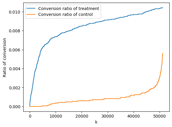
Similarly, we can also compute and plot the conversion ratio of those not receiving an email, called the control group. Ideally, this curve is initially flat: This would mean that the model does not prioritize sending emails to clients that will generate a conversion despite not receiving a email

ratio_control = np.cumsum(np.multiply(outcomes_sorted, control_sorted), axis=0)/num_control
ax.plot(ratio_control, label='Conversion ratio of control')
ax.legend()
fig

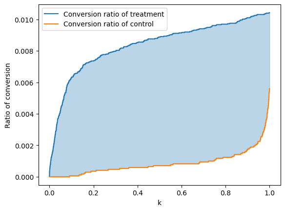
The AUUC metric measures the area between these two curves, normalizing the y-axis between 0 and 1

x = np.linspace(0, 1, num_examples)
plt.plot(x,ratio_treatment, label='Conversion ratio of treatment')
plt.plot(x,ratio_control, label='Conversion ratio of control')
plt.fill_between(x, ratio_treatment, ratio_control, where=(ratio_treatment > ratio_control), color='C0', alpha=0.3)
plt.fill_between(x, ratio_treatment, ratio_control, where=(ratio_treatment < ratio_control), color='C1', alpha=0.3)
plt.xlabel('k')
plt.ylabel('Ratio of conversion')
plt.legend()

# Approximate the integral of the difference between the two curves.
auuc = np.trapz(ratio_treatment-ratio_control, dx=1/num_examples)
print(f'The AUUC on the test dataset is {auuc}')

/tmpfs/tmp/ipykernel_9083/1475983573.py:11: DeprecationWarning: `trapz` is deprecated. Use `trapezoid` instead, or one of the numerical integration functions in `scipy.integrate`.
  auuc = np.trapz(ratio_treatment-ratio_control, dx=1/num_examples)
The AUUC on the test dataset is 0.007513949426065613