
| | |  GitHub에서 소스 보기 GitHub에서 소스 보기 | |
이 튜토리얼은 Tensorflow Federated를 사용하여 사용자 수준의 차등 개인정보 보호를 사용하여 모델을 교육하는 데 권장되는 모범 사례를 보여줍니다. 우리의 DP-SGD 알고리즘을 사용합니다 아 바디 등. "차등 개인 정보 보호와 깊은 학습" 에 페더 레이 티드 환경에서 사용자 수준 DP에 대한 수정 McMahan 등., "학습 된 유의 개인 재발 언어 모델" .
DP(Differential Privacy)는 학습 작업을 수행할 때 민감한 데이터의 개인 정보 유출을 제한하고 수량화하는 데 널리 사용되는 방법입니다. 사용자 수준 DP로 모델을 훈련하면 모델이 개인의 데이터에 대해 중요한 것을 학습할 가능성은 거의 없지만 많은 클라이언트의 데이터에 존재하는 패턴을 계속 학습할 수 있습니다.
연합된 EMNIST 데이터 세트에서 모델을 훈련할 것입니다. 효용과 개인 정보 보호 간에는 고유한 절충점이 있으며, 최신 비개인 모델만큼 성능이 우수한 개인 정보 보호 수준이 높은 모델을 훈련시키는 것은 어려울 수 있습니다. 이 튜토리얼에서는 편의를 위해 100라운드 동안만 훈련하고 높은 개인 정보 보호를 사용하여 훈련하는 방법을 보여주기 위해 일부 품질을 희생합니다. 더 많은 훈련 라운드를 사용한다면 확실히 다소 더 높은 정확도의 개인 모델을 가질 수 있지만 DP 없이 훈련된 모델만큼 높지는 않습니다.
시작하기 전에
먼저 노트북이 관련 구성 요소가 컴파일된 백엔드에 연결되어 있는지 확인합니다.
!pip install --quiet --upgrade tensorflow_federated_nightly
!pip install --quiet --upgrade nest-asyncio

import nest_asyncio
nest_asyncio.apply()
튜토리얼에 필요한 일부 가져오기. 우리는 사용 tensorflow_federated , 기계 학습 및 분산 데이터에 대한 다른 계산뿐만 아니라위한 오픈 소스 프레임 워크 tensorflow_privacy , 구현하고 tensorflow에 차등 개인 알고리즘 분석을위한 오픈 소스 라이브러리를.
import collections

import numpy as np
import pandas as pd
import tensorflow as tf
import tensorflow_federated as tff
import tensorflow_privacy as tfp
다음 "Hello World" 예제를 실행하여 TFF 환경이 올바르게 설정되었는지 확인하십시오. 그것이 작동하지 않는 경우를 참조하십시오 설치 지침은 가이드.
@tff.federated_computation
def hello_world():
  return 'Hello, World!'

hello_world()
b'Hello, World!'
연합 EMNIST 데이터 세트를 다운로드하고 사전 처리합니다.
def get_emnist_dataset():
  emnist_train, emnist_test = tff.simulation.datasets.emnist.load_data(
      only_digits=True)

  def element_fn(element):
    return collections.OrderedDict(
        x=tf.expand_dims(element['pixels'], -1), y=element['label'])

  def preprocess_train_dataset(dataset):
    # Use buffer_size same as the maximum client dataset size,
    # 418 for Federated EMNIST
    return (dataset.map(element_fn)
                   .shuffle(buffer_size=418)
                   .repeat(1)
                   .batch(32, drop_remainder=False))

  def preprocess_test_dataset(dataset):
    return dataset.map(element_fn).batch(128, drop_remainder=False)

  emnist_train = emnist_train.preprocess(preprocess_train_dataset)
  emnist_test = preprocess_test_dataset(
      emnist_test.create_tf_dataset_from_all_clients())
  return emnist_train, emnist_test

train_data, test_data = get_emnist_dataset()
우리의 모델을 정의하십시오.
def my_model_fn():
  model = tf.keras.models.Sequential([
      tf.keras.layers.Reshape(input_shape=(28, 28, 1), target_shape=(28 * 28,)),
      tf.keras.layers.Dense(200, activation=tf.nn.relu),
      tf.keras.layers.Dense(200, activation=tf.nn.relu),
      tf.keras.layers.Dense(10)])
  return tff.learning.from_keras_model(
      keras_model=model,
      loss=tf.keras.losses.SparseCategoricalCrossentropy(from_logits=True),
      input_spec=test_data.element_spec,
      metrics=[tf.keras.metrics.SparseCategoricalAccuracy()])
모델의 노이즈 감도를 결정합니다.
사용자 수준의 DP 보장을 얻으려면 기본 Federated Averaging 알고리즘을 두 가지 방식으로 변경해야 합니다. 첫째, 클라이언트의 모델 업데이트는 서버로 전송하기 전에 잘려서 한 클라이언트의 최대 영향을 제한해야 합니다. 둘째, 서버는 최악의 경우 클라이언트 영향을 모호하게 하기 위해 평균화하기 전에 사용자 업데이트 합계에 충분한 노이즈를 추가해야 합니다.
클리핑을 위해, 우리는의 적응 클리핑 방법을 사용 앤드류 외. 2021, 어댑티브 패스 된 유의 개인 학습은 어떤 클리핑 규범이 필요하지 않도록 명시 적으로 설정합니다.
노이즈를 추가하면 일반적으로 모델의 효용이 저하되지만 두 개의 노브를 사용하여 각 라운드에서 평균 업데이트의 노이즈 양을 제어할 수 있습니다. 합계에 추가된 가우스 노이즈의 표준 편차와 평균. 우리의 전략은 먼저 모델 유틸리티에 대한 허용 가능한 손실과 함께 라운드당 비교적 적은 수의 클라이언트에서 모델이 견딜 수 있는 소음의 양을 결정하는 것입니다. 그런 다음 최종 모델을 훈련하기 위해 합계에서 노이즈의 양을 늘리면서 라운드당 클라이언트 수를 비례적으로 확장할 수 있습니다(데이터 세트가 라운드당 많은 클라이언트를 지원할 만큼 충분히 크다고 가정). 유일한 효과는 클라이언트 샘플링으로 인한 분산을 줄이는 것뿐이므로 모델 품질에 큰 영향을 미치지 않을 것입니다(실제로 우리의 경우에는 그렇지 않음을 확인할 것입니다).
이를 위해 먼저 라운드당 50명의 클라이언트가 있는 일련의 모델을 훈련하고 노이즈 양을 증가시킵니다. 특히 노이즈 표준 편차와 클리핑 놈의 비율인 "noise_multiplier"를 높입니다. 적응형 클리핑을 사용하기 때문에 노이즈의 실제 크기가 라운드에서 라운드로 변경됩니다.
# Run five clients per thread. Increase this if your runtime is running out of
# memory. Decrease it if you have the resources and want to speed up execution.
tff.backends.native.set_local_python_execution_context(clients_per_thread=5)

total_clients = len(train_data.client_ids)

def train(rounds, noise_multiplier, clients_per_round, data_frame):
  # Using the `dp_aggregator` here turns on differential privacy with adaptive
  # clipping.
  aggregation_factory = tff.learning.model_update_aggregator.dp_aggregator(
      noise_multiplier, clients_per_round)

  # We use Poisson subsampling which gives slightly tighter privacy guarantees
  # compared to having a fixed number of clients per round. The actual number of
  # clients per round is stochastic with mean clients_per_round.
  sampling_prob = clients_per_round / total_clients

  # Build a federated averaging process.
  # Typically a non-adaptive server optimizer is used because the noise in the
  # updates can cause the second moment accumulators to become very large
  # prematurely.
  learning_process = tff.learning.build_federated_averaging_process(
        my_model_fn,
        client_optimizer_fn=lambda: tf.keras.optimizers.SGD(0.01),
        server_optimizer_fn=lambda: tf.keras.optimizers.SGD(1.0, momentum=0.9),
        model_update_aggregation_factory=aggregation_factory)

  eval_process = tff.learning.build_federated_evaluation(my_model_fn)

  # Training loop.
  state = learning_process.initialize()
  for round in range(rounds):
    if round % 5 == 0:
      metrics = eval_process(state.model, [test_data])['eval']
      if round < 25 or round % 25 == 0:
        print(f'Round {round:3d}: {metrics}')
      data_frame = data_frame.append({'Round': round,
                                      'NoiseMultiplier': noise_multiplier,
                                      **metrics}, ignore_index=True)

    # Sample clients for a round. Note that if your dataset is large and
    # sampling_prob is small, it would be faster to use gap sampling.
    x = np.random.uniform(size=total_clients)
    sampled_clients = [
        train_data.client_ids[i] for i in range(total_clients)
        if x[i] < sampling_prob]
    sampled_train_data = [
        train_data.create_tf_dataset_for_client(client)
        for client in sampled_clients]

    # Use selected clients for update.
    state, metrics = learning_process.next(state, sampled_train_data)

  metrics = eval_process(state.model, [test_data])['eval']
  print(f'Round {rounds:3d}: {metrics}')
  data_frame = data_frame.append({'Round': rounds,
                                  'NoiseMultiplier': noise_multiplier,
                                  **metrics}, ignore_index=True)

  return data_frame
data_frame = pd.DataFrame()
rounds = 100
clients_per_round = 50

for noise_multiplier in [0.0, 0.5, 0.75, 1.0]:
  print(f'Starting training with noise multiplier: {noise_multiplier}')
  data_frame = train(rounds, noise_multiplier, clients_per_round, data_frame)
  print()
Starting training with noise multiplier: 0.0
Round   0: OrderedDict([('sparse_categorical_accuracy', 0.112289384), ('loss', 2.5190482)])
Round   5: OrderedDict([('sparse_categorical_accuracy', 0.19075724), ('loss', 2.2449977)])
Round  10: OrderedDict([('sparse_categorical_accuracy', 0.18115693), ('loss', 2.163907)])
Round  15: OrderedDict([('sparse_categorical_accuracy', 0.49970612), ('loss', 2.01017)])
Round  20: OrderedDict([('sparse_categorical_accuracy', 0.5333317), ('loss', 1.8350543)])
Round  25: OrderedDict([('sparse_categorical_accuracy', 0.5828517), ('loss', 1.6551636)])
Round  50: OrderedDict([('sparse_categorical_accuracy', 0.7352077), ('loss', 0.8700141)])
Round  75: OrderedDict([('sparse_categorical_accuracy', 0.7769152), ('loss', 0.6992781)])
Round 100: OrderedDict([('sparse_categorical_accuracy', 0.8049814), ('loss', 0.62453026)])

Starting training with noise multiplier: 0.5
Round   0: OrderedDict([('sparse_categorical_accuracy', 0.09526841), ('loss', 2.4332638)])
Round   5: OrderedDict([('sparse_categorical_accuracy', 0.20128821), ('loss', 2.2664592)])
Round  10: OrderedDict([('sparse_categorical_accuracy', 0.35472178), ('loss', 2.130336)])
Round  15: OrderedDict([('sparse_categorical_accuracy', 0.5480995), ('loss', 1.9713942)])
Round  20: OrderedDict([('sparse_categorical_accuracy', 0.42246276), ('loss', 1.8045483)])
Round  25: OrderedDict([('sparse_categorical_accuracy', 0.624902), ('loss', 1.4785467)])
Round  50: OrderedDict([('sparse_categorical_accuracy', 0.7265625), ('loss', 0.85801566)])
Round  75: OrderedDict([('sparse_categorical_accuracy', 0.77720904), ('loss', 0.70615387)])
Round 100: OrderedDict([('sparse_categorical_accuracy', 0.7702537), ('loss', 0.72331005)])

Starting training with noise multiplier: 0.75
Round   0: OrderedDict([('sparse_categorical_accuracy', 0.098672606), ('loss', 2.422002)])
Round   5: OrderedDict([('sparse_categorical_accuracy', 0.11794671), ('loss', 2.2227976)])
Round  10: OrderedDict([('sparse_categorical_accuracy', 0.3208513), ('loss', 2.083766)])
Round  15: OrderedDict([('sparse_categorical_accuracy', 0.49752644), ('loss', 1.8728142)])
Round  20: OrderedDict([('sparse_categorical_accuracy', 0.5816761), ('loss', 1.6084186)])
Round  25: OrderedDict([('sparse_categorical_accuracy', 0.62896746), ('loss', 1.378527)])
Round  50: OrderedDict([('sparse_categorical_accuracy', 0.73153406), ('loss', 0.8705139)])
Round  75: OrderedDict([('sparse_categorical_accuracy', 0.7789724), ('loss', 0.7113147)])
Round 100: OrderedDict([('sparse_categorical_accuracy', 0.70944357), ('loss', 0.89495045)])

Starting training with noise multiplier: 1.0
Round   0: OrderedDict([('sparse_categorical_accuracy', 0.12002841), ('loss', 2.60482)])
Round   5: OrderedDict([('sparse_categorical_accuracy', 0.104574844), ('loss', 2.3388205)])
Round  10: OrderedDict([('sparse_categorical_accuracy', 0.29966694), ('loss', 2.089262)])
Round  15: OrderedDict([('sparse_categorical_accuracy', 0.4067398), ('loss', 1.9109797)])
Round  20: OrderedDict([('sparse_categorical_accuracy', 0.5123677), ('loss', 1.6472703)])
Round  25: OrderedDict([('sparse_categorical_accuracy', 0.56416535), ('loss', 1.4362282)])
Round  50: OrderedDict([('sparse_categorical_accuracy', 0.62323666), ('loss', 1.1682972)])
Round  75: OrderedDict([('sparse_categorical_accuracy', 0.55968356), ('loss', 1.4779186)])
Round 100: OrderedDict([('sparse_categorical_accuracy', 0.382837), ('loss', 1.9680436)])
이제 평가 세트 정확도와 해당 실행의 손실을 시각화할 수 있습니다.
import matplotlib.pyplot as plt
import seaborn as sns

def make_plot(data_frame):
  plt.figure(figsize=(15, 5))

  dff = data_frame.rename(
      columns={'sparse_categorical_accuracy': 'Accuracy', 'loss': 'Loss'})

  plt.subplot(121)
  sns.lineplot(data=dff, x='Round', y='Accuracy', hue='NoiseMultiplier', palette='dark')
  plt.subplot(122)
  sns.lineplot(data=dff, x='Round', y='Loss', hue='NoiseMultiplier', palette='dark')
make_plot(data_frame)
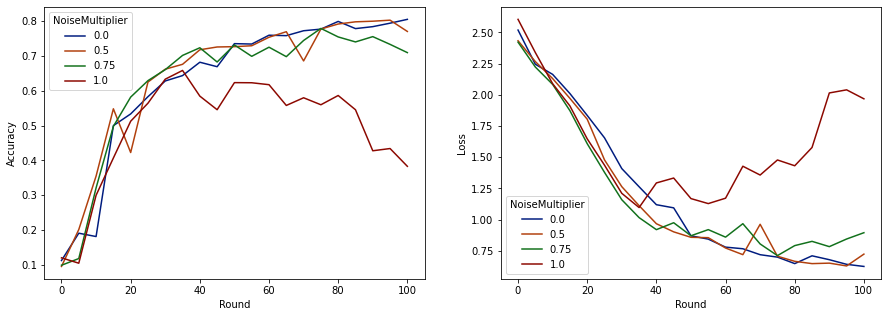
라운드당 50명의 예상 클라이언트가 있는 이 모델은 모델 품질을 저하시키지 않으면서 최대 0.5의 노이즈 승수를 견딜 수 있는 것으로 보입니다. 0.75의 노이즈 승수는 약간의 모델 저하를 일으키는 것으로 보이며 1.0은 모델을 발산합니다.
일반적으로 모델 품질과 개인 정보 보호 간에는 절충점이 있습니다. 노이즈를 많이 사용할수록 동일한 교육 시간과 클라이언트 수에 대해 더 많은 개인 정보를 얻을 수 있습니다. 반대로 노이즈가 적으면 더 정확한 모델을 가질 수 있지만 목표 개인 정보 보호 수준에 도달하려면 라운드당 더 많은 클라이언트로 훈련해야 합니다.
위의 실험을 통해 최종 모델을 더 빠르게 훈련시키기 위해 0.75에서 약간의 모델 열화가 허용된다고 결정할 수 있지만 0.5 노이즈 승수 모델의 성능과 일치시키길 원한다고 가정해 보겠습니다.
이제 tensorflow_privacy 함수를 사용하여 허용 가능한 개인 정보를 얻는 데 필요한 라운드당 예상 클라이언트 수를 결정할 수 있습니다. 표준 관행은 데이터 세트의 레코드 수보다 1보다 약간 작은 델타를 선택하는 것입니다. 이 데이터 세트에는 총 3383명의 훈련 사용자가 있으므로 (2, 1e-5)-DP를 목표로 합시다.
라운드당 클라이언트 수에 대해 간단한 이진 검색을 사용합니다. 우리는, ε을 추정하기 위해 사용하는 tensorflow_privacy 함수에 기초 왕 등. (2018) 및 미로 노프 등. (2019) .
rdp_orders = ([1.25, 1.5, 1.75, 2., 2.25, 2.5, 3., 3.5, 4., 4.5] +
              list(range(5, 64)) + [128, 256, 512])

total_clients = 3383
base_noise_multiplier = 0.5
base_clients_per_round = 50
target_delta = 1e-5
target_eps = 2

def get_epsilon(clients_per_round):
  # If we use this number of clients per round and proportionally
  # scale up the noise multiplier, what epsilon do we achieve?
  q = clients_per_round / total_clients
  noise_multiplier = base_noise_multiplier
  noise_multiplier *= clients_per_round / base_clients_per_round
  rdp = tfp.compute_rdp(
      q, noise_multiplier=noise_multiplier, steps=rounds, orders=rdp_orders)
  eps, _, _ = tfp.get_privacy_spent(rdp_orders, rdp, target_delta=target_delta)
  return clients_per_round, eps, noise_multiplier

def find_needed_clients_per_round():
  hi = get_epsilon(base_clients_per_round)
  if hi[1] < target_eps:
    return hi

  # Grow interval exponentially until target_eps is exceeded.
  while True:
    lo = hi
    hi = get_epsilon(2 * lo[0])
    if hi[1] < target_eps:
      break

  # Binary search.
  while hi[0] - lo[0] > 1:
    mid = get_epsilon((lo[0] + hi[0]) // 2)
    if mid[1] > target_eps:
      lo = mid
    else:
      hi = mid

  return hi

clients_per_round, _, noise_multiplier = find_needed_clients_per_round()
print(f'To get ({target_eps}, {target_delta})-DP, use {clients_per_round} '
      f'clients with noise multiplier {noise_multiplier}.')
To get (2, 1e-05)-DP, use 120 clients with noise multiplier 1.2.
이제 출시를 위해 최종 비공개 모델을 훈련할 수 있습니다.
rounds = 100
noise_multiplier = 1.2
clients_per_round = 120

data_frame = pd.DataFrame()
data_frame = train(rounds, noise_multiplier, clients_per_round, data_frame)

make_plot(data_frame)
Round   0: OrderedDict([('sparse_categorical_accuracy', 0.08260678), ('loss', 2.6334999)])
Round   5: OrderedDict([('sparse_categorical_accuracy', 0.1492212), ('loss', 2.259542)])
Round  10: OrderedDict([('sparse_categorical_accuracy', 0.28847474), ('loss', 2.155699)])
Round  15: OrderedDict([('sparse_categorical_accuracy', 0.3989518), ('loss', 2.0156953)])
Round  20: OrderedDict([('sparse_categorical_accuracy', 0.5086697), ('loss', 1.8261365)])
Round  25: OrderedDict([('sparse_categorical_accuracy', 0.6204692), ('loss', 1.5602393)])
Round  50: OrderedDict([('sparse_categorical_accuracy', 0.70008814), ('loss', 0.91155165)])
Round  75: OrderedDict([('sparse_categorical_accuracy', 0.78421336), ('loss', 0.6820159)])
Round 100: OrderedDict([('sparse_categorical_accuracy', 0.7955525), ('loss', 0.6585961)])
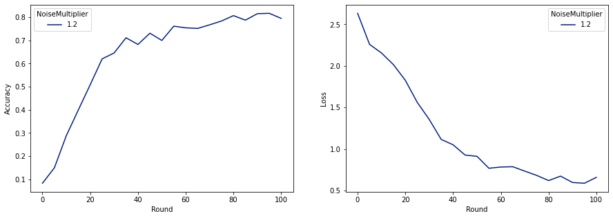
보시다시피 최종 모델은 노이즈 없이 훈련된 모델과 손실과 정확도가 비슷하지만 (2, 1e-5)-DP를 만족합니다.