| | |  ดูแหล่งที่มาบน GitHub ดูแหล่งที่มาบน GitHub | |
ภาพรวม
เครื่องประมาณค่าแบบกระป๋องเป็นวิธีที่ง่ายและรวดเร็วในการฝึกโมเดล TFL สำหรับกรณีการใช้งานทั่วไป คู่มือนี้สรุปขั้นตอนที่จำเป็นในการสร้างตัวประมาณค่า TFL แบบบรรจุกระป๋อง
ติดตั้ง
การติดตั้งแพ็คเกจ TF Lattice:
pip install tensorflow-lattice
การนำเข้าแพ็คเกจที่จำเป็น:
import tensorflow as tf

import copy
import logging
import numpy as np
import pandas as pd
import sys
import tensorflow_lattice as tfl
from tensorflow import feature_column as fc
logging.disable(sys.maxsize)
กำลังดาวน์โหลดชุดข้อมูล UCI Statlog (หัวใจ):
csv_file = tf.keras.utils.get_file(
    'heart.csv', 'http://storage.googleapis.com/download.tensorflow.org/data/heart.csv')
df = pd.read_csv(csv_file)
target = df.pop('target')
train_size = int(len(df) * 0.8)
train_x = df[:train_size]
train_y = target[:train_size]
test_x = df[train_size:]
test_y = target[train_size:]
df.head()
การตั้งค่าเริ่มต้นที่ใช้สำหรับการฝึกอบรมในคู่มือนี้:
LEARNING_RATE = 0.01
BATCH_SIZE = 128
NUM_EPOCHS = 500
PREFITTING_NUM_EPOCHS = 10
คอลัมน์คุณลักษณะ
สำหรับประมาณการ TF อื่น ๆ ความต้องการข้อมูลที่จะส่งผ่านไปยังประมาณการซึ่งโดยปกติจะผ่าน input_fn และแยกวิเคราะห์โดยใช้ FeatureColumns
# Feature columns.
# - age
# - sex
# - cp        chest pain type (4 values)
# - trestbps  resting blood pressure
# - chol      serum cholestoral in mg/dl
# - fbs       fasting blood sugar > 120 mg/dl
# - restecg   resting electrocardiographic results (values 0,1,2)
# - thalach   maximum heart rate achieved
# - exang     exercise induced angina
# - oldpeak   ST depression induced by exercise relative to rest
# - slope     the slope of the peak exercise ST segment
# - ca        number of major vessels (0-3) colored by flourosopy
# - thal      3 = normal; 6 = fixed defect; 7 = reversable defect
feature_columns = [
    fc.numeric_column('age', default_value=-1),
    fc.categorical_column_with_vocabulary_list('sex', [0, 1]),
    fc.numeric_column('cp'),
    fc.numeric_column('trestbps', default_value=-1),
    fc.numeric_column('chol'),
    fc.categorical_column_with_vocabulary_list('fbs', [0, 1]),
    fc.categorical_column_with_vocabulary_list('restecg', [0, 1, 2]),
    fc.numeric_column('thalach'),
    fc.categorical_column_with_vocabulary_list('exang', [0, 1]),
    fc.numeric_column('oldpeak'),
    fc.categorical_column_with_vocabulary_list('slope', [0, 1, 2]),
    fc.numeric_column('ca'),
    fc.categorical_column_with_vocabulary_list(
        'thal', ['normal', 'fixed', 'reversible']),
]
เครื่องมือประมาณค่าแบบกระป๋อง TFL ใช้ประเภทของคอลัมน์คุณลักษณะเพื่อตัดสินใจว่าจะใช้ชั้นการสอบเทียบประเภทใด เราใช้ tfl.layers.PWLCalibration ชั้นสำหรับคอลัมน์คุณลักษณะที่เป็นตัวเลขและ tfl.layers.CategoricalCalibration ชั้นสำหรับคอลัมน์คุณลักษณะเด็ดขาด
โปรดทราบว่าคอลัมน์คุณลักษณะตามหมวดหมู่ไม่ได้ครอบคลุมคอลัมน์คุณลักษณะการฝัง พวกมันจะถูกป้อนเข้าสู่ตัวประมาณโดยตรง
กำลังสร้าง input_fn
สำหรับตัวประมาณอื่นๆ คุณสามารถใช้ input_fn เพื่อป้อนข้อมูลไปยังแบบจำลองสำหรับการฝึกอบรมและการประเมิน ตัวประมาณค่า TFL สามารถคำนวณปริมาณของคุณสมบัติได้โดยอัตโนมัติและใช้เป็นคีย์พอยท์อินพุตสำหรับเลเยอร์การสอบเทียบ PWL ที่จะทำเช่นนั้นพวกเขาต้องผ่าน feature_analysis_input_fn ซึ่งมีลักษณะคล้ายกับการฝึกอบรม input_fn แต่ด้วยยุคเดียวหรือ subsample ของข้อมูลที่
train_input_fn = tf.compat.v1.estimator.inputs.pandas_input_fn(
    x=train_x,
    y=train_y,
    shuffle=False,
    batch_size=BATCH_SIZE,
    num_epochs=NUM_EPOCHS,
    num_threads=1)

# feature_analysis_input_fn is used to collect statistics about the input.
feature_analysis_input_fn = tf.compat.v1.estimator.inputs.pandas_input_fn(
    x=train_x,
    y=train_y,
    shuffle=False,
    batch_size=BATCH_SIZE,
    # Note that we only need one pass over the data.
    num_epochs=1,
    num_threads=1)

test_input_fn = tf.compat.v1.estimator.inputs.pandas_input_fn(
    x=test_x,
    y=test_y,
    shuffle=False,
    batch_size=BATCH_SIZE,
    num_epochs=1,
    num_threads=1)

# Serving input fn is used to create saved models.
serving_input_fn = (
    tf.estimator.export.build_parsing_serving_input_receiver_fn(
        feature_spec=fc.make_parse_example_spec(feature_columns)))
การกำหนดค่าคุณสมบัติ
การกำหนดค่าการสอบเทียบบาร์และต่อคุณลักษณะที่มีการตั้งค่าการใช้ tfl.configs.FeatureConfig การกำหนดค่าคุณลักษณะรวมถึงข้อ จำกัด monotonicity, กูต่อคุณลักษณะ (ดู tfl.configs.RegularizerConfig ) และขนาดตาข่ายสำหรับรูปแบบตาข่าย
หากไม่มีการกำหนดค่าที่กำหนดไว้สำหรับคุณลักษณะการป้อนข้อมูลการตั้งค่าเริ่มต้นใน tfl.config.FeatureConfig ถูกนำมาใช้
# Feature configs are used to specify how each feature is calibrated and used.
feature_configs = [
    tfl.configs.FeatureConfig(
        name='age',
        lattice_size=3,
        # By default, input keypoints of pwl are quantiles of the feature.
        pwl_calibration_num_keypoints=5,
        monotonicity='increasing',
        pwl_calibration_clip_max=100,
        # Per feature regularization.
        regularizer_configs=[
            tfl.configs.RegularizerConfig(name='calib_wrinkle', l2=0.1),
        ],
    ),
    tfl.configs.FeatureConfig(
        name='cp',
        pwl_calibration_num_keypoints=4,
        # Keypoints can be uniformly spaced.
        pwl_calibration_input_keypoints='uniform',
        monotonicity='increasing',
    ),
    tfl.configs.FeatureConfig(
        name='chol',
        # Explicit input keypoint initialization.
        pwl_calibration_input_keypoints=[126.0, 210.0, 247.0, 286.0, 564.0],
        monotonicity='increasing',
        # Calibration can be forced to span the full output range by clamping.
        pwl_calibration_clamp_min=True,
        pwl_calibration_clamp_max=True,
        # Per feature regularization.
        regularizer_configs=[
            tfl.configs.RegularizerConfig(name='calib_hessian', l2=1e-4),
        ],
    ),
    tfl.configs.FeatureConfig(
        name='fbs',
        # Partial monotonicity: output(0) <= output(1)
        monotonicity=[(0, 1)],
    ),
    tfl.configs.FeatureConfig(
        name='trestbps',
        pwl_calibration_num_keypoints=5,
        monotonicity='decreasing',
    ),
    tfl.configs.FeatureConfig(
        name='thalach',
        pwl_calibration_num_keypoints=5,
        monotonicity='decreasing',
    ),
    tfl.configs.FeatureConfig(
        name='restecg',
        # Partial monotonicity: output(0) <= output(1), output(0) <= output(2)
        monotonicity=[(0, 1), (0, 2)],
    ),
    tfl.configs.FeatureConfig(
        name='exang',
        # Partial monotonicity: output(0) <= output(1)
        monotonicity=[(0, 1)],
    ),
    tfl.configs.FeatureConfig(
        name='oldpeak',
        pwl_calibration_num_keypoints=5,
        monotonicity='increasing',
    ),
    tfl.configs.FeatureConfig(
        name='slope',
        # Partial monotonicity: output(0) <= output(1), output(1) <= output(2)
        monotonicity=[(0, 1), (1, 2)],
    ),
    tfl.configs.FeatureConfig(
        name='ca',
        pwl_calibration_num_keypoints=4,
        monotonicity='increasing',
    ),
    tfl.configs.FeatureConfig(
        name='thal',
        # Partial monotonicity:
        # output(normal) <= output(fixed)
        # output(normal) <= output(reversible)
        monotonicity=[('normal', 'fixed'), ('normal', 'reversible')],
    ),
]
แบบจำลองเชิงเส้นที่สอบเทียบ
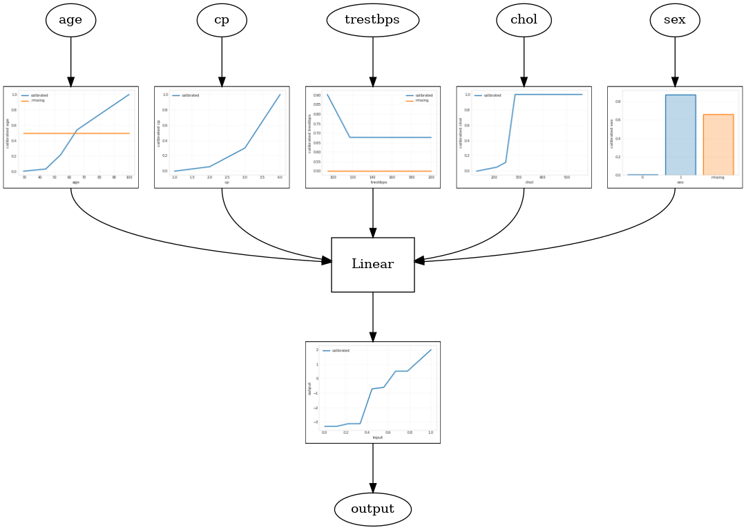
เพื่อสร้าง TFL กระป๋องประมาณการสร้างการตั้งค่ารูปแบบจาก tfl.configs ปรับเทียบแบบจำลองเชิงเส้นจะถูกสร้างขึ้นโดยใช้ tfl.configs.CalibratedLinearConfig ใช้การสอบเทียบทีละชิ้นและตามหมวดหมู่กับคุณสมบัติอินพุต ตามด้วยการผสมผสานเชิงเส้นและการสอบเทียบเอาต์พุตแบบแยกชิ้น-เชิงเส้นที่เป็นตัวเลือก เมื่อใช้การปรับเทียบเอาต์พุตหรือเมื่อกำหนดขอบเขตเอาต์พุต เลเยอร์เชิงเส้นจะใช้การถัวเฉลี่ยถ่วงน้ำหนักกับอินพุตที่ปรับเทียบแล้ว
ตัวอย่างนี้สร้างแบบจำลองเชิงเส้นตรงที่ปรับเทียบแล้วใน 5 คุณลักษณะแรก เราใช้ tfl.visualization พล็อตกราฟรุ่นที่มีแผนการสอบเทียบ
# Model config defines the model structure for the estimator.
model_config = tfl.configs.CalibratedLinearConfig(
    feature_configs=feature_configs,
    use_bias=True,
    output_calibration=True,
    regularizer_configs=[
        # Regularizer for the output calibrator.
        tfl.configs.RegularizerConfig(name='output_calib_hessian', l2=1e-4),
    ])
# A CannedClassifier is constructed from the given model config.
estimator = tfl.estimators.CannedClassifier(
    feature_columns=feature_columns[:5],
    model_config=model_config,
    feature_analysis_input_fn=feature_analysis_input_fn,
    optimizer=tf.keras.optimizers.Adam(LEARNING_RATE),
    config=tf.estimator.RunConfig(tf_random_seed=42))
estimator.train(input_fn=train_input_fn)
results = estimator.evaluate(input_fn=test_input_fn)
print('Calibrated linear test AUC: {}'.format(results['auc']))
saved_model_path = estimator.export_saved_model(estimator.model_dir,
                                                serving_input_fn)
model_graph = tfl.estimators.get_model_graph(saved_model_path)
tfl.visualization.draw_model_graph(model_graph)
2021-09-30 20:54:06.660239: E tensorflow/stream_executor/cuda/cuda_driver.cc:271] failed call to cuInit: CUDA_ERROR_NO_DEVICE: no CUDA-capable device is detected
Calibrated linear test AUC: 0.834586501121521
แบบจำลอง Lattice ที่ปรับเทียบแล้ว
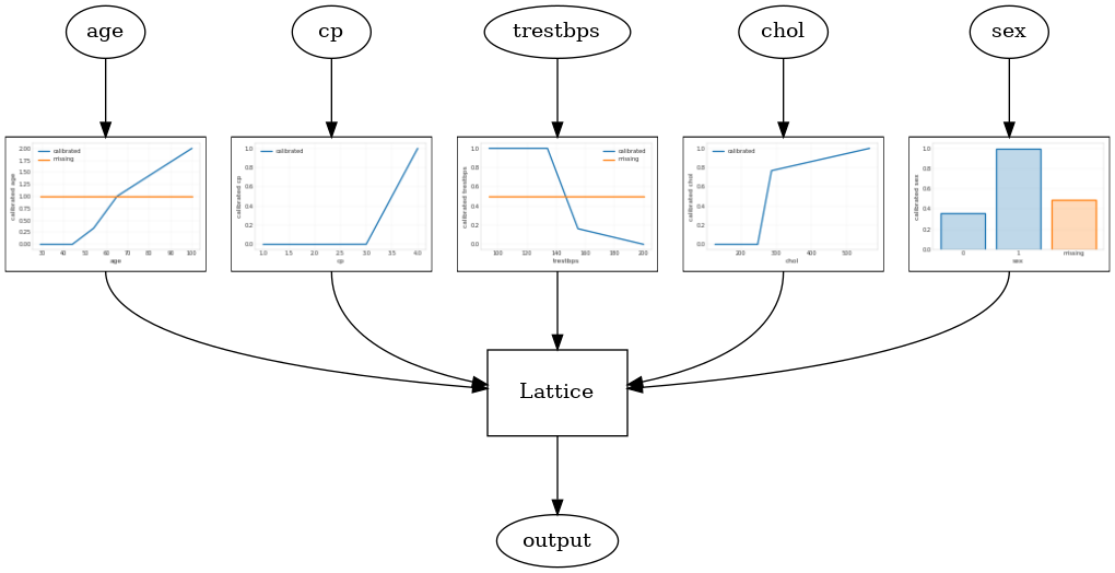
สอบเทียบรุ่นตาข่ายถูกสร้างโดยใช้ tfl.configs.CalibratedLatticeConfig โมเดลแลตทิซที่ปรับเทียบแล้วจะใช้การสอบเทียบแบบทีละชิ้นและแบบตามหมวดหมู่กับคุณสมบัติอินพุต ตามด้วยแบบจำลองแลตทิซและการสอบเทียบเอาต์พุตแบบทีละชิ้นซึ่งเป็นตัวเลือกเสริม
ตัวอย่างนี้สร้างแบบจำลองแลตทิซที่ปรับเทียบแล้วใน 5 คุณสมบัติแรก
# This is calibrated lattice model: Inputs are calibrated, then combined
# non-linearly using a lattice layer.
model_config = tfl.configs.CalibratedLatticeConfig(
    feature_configs=feature_configs,
    regularizer_configs=[
        # Torsion regularizer applied to the lattice to make it more linear.
        tfl.configs.RegularizerConfig(name='torsion', l2=1e-4),
        # Globally defined calibration regularizer is applied to all features.
        tfl.configs.RegularizerConfig(name='calib_hessian', l2=1e-4),
    ])
# A CannedClassifier is constructed from the given model config.
estimator = tfl.estimators.CannedClassifier(
    feature_columns=feature_columns[:5],
    model_config=model_config,
    feature_analysis_input_fn=feature_analysis_input_fn,
    optimizer=tf.keras.optimizers.Adam(LEARNING_RATE),
    config=tf.estimator.RunConfig(tf_random_seed=42))
estimator.train(input_fn=train_input_fn)
results = estimator.evaluate(input_fn=test_input_fn)
print('Calibrated lattice test AUC: {}'.format(results['auc']))
saved_model_path = estimator.export_saved_model(estimator.model_dir,
                                                serving_input_fn)
model_graph = tfl.estimators.get_model_graph(saved_model_path)
tfl.visualization.draw_model_graph(model_graph)
Calibrated lattice test AUC: 0.8427318930625916
สอบเทียบ Lattice Ensemble
เมื่อฟีเจอร์มีจำนวนมาก คุณสามารถใช้โมเดลทั้งมวล ซึ่งสร้างแลตทิซขนาดเล็กกว่าหลายอันสำหรับชุดย่อยของฟีเจอร์และหาค่าเฉลี่ยของเอาต์พุต แทนที่จะสร้างเพียงแลตทิซขนาดใหญ่เพียงอันเดียว รุ่นตาข่ายทั้งมวลจะถูกสร้างขึ้นโดยใช้ tfl.configs.CalibratedLatticeEnsembleConfig รุ่นชุดขัดแตะขัดแตะที่ปรับเทียบแล้วจะใช้การปรับเทียบทีละชิ้นและตามหมวดหมู่กับคุณสมบัติอินพุต ตามด้วยชุดของรุ่นขัดแตะและการปรับเทียบเอาต์พุตแบบแยกชิ้น-เส้นตรงที่เป็นอุปกรณ์เสริม
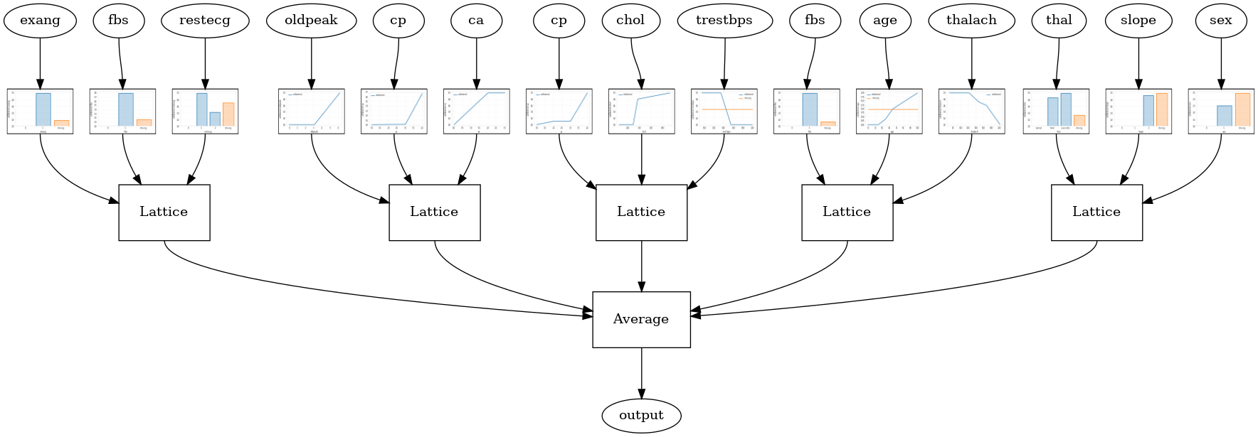
สุ่ม Lattice Ensemble
การกำหนดค่าโมเดลต่อไปนี้ใช้ชุดย่อยของคุณลักษณะแบบสุ่มสำหรับแต่ละโครงข่าย
# This is random lattice ensemble model with separate calibration:
# model output is the average output of separately calibrated lattices.
model_config = tfl.configs.CalibratedLatticeEnsembleConfig(
    feature_configs=feature_configs,
    num_lattices=5,
    lattice_rank=3)
# A CannedClassifier is constructed from the given model config.
estimator = tfl.estimators.CannedClassifier(
    feature_columns=feature_columns,
    model_config=model_config,
    feature_analysis_input_fn=feature_analysis_input_fn,
    optimizer=tf.keras.optimizers.Adam(LEARNING_RATE),
    config=tf.estimator.RunConfig(tf_random_seed=42))
estimator.train(input_fn=train_input_fn)
results = estimator.evaluate(input_fn=test_input_fn)
print('Random ensemble test AUC: {}'.format(results['auc']))
saved_model_path = estimator.export_saved_model(estimator.model_dir,
                                                serving_input_fn)
model_graph = tfl.estimators.get_model_graph(saved_model_path)
tfl.visualization.draw_model_graph(model_graph, calibrator_dpi=15)
Random ensemble test AUC: 0.9003759026527405
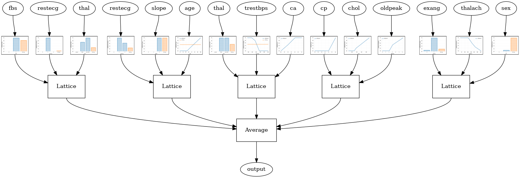
RTL Layer Random Lattice Ensemble
กำหนดค่ารูปแบบต่อไปนี้ใช้ tfl.layers.RTL ชั้นที่ใช้เซตสุ่มของคุณสมบัติสำหรับแต่ละตาข่าย เราทราบว่า tfl.layers.RTL สนับสนุนเฉพาะข้อ จำกัด monotonicity และต้องมีขนาดตาข่ายเหมือนกันสำหรับคุณสมบัติและไม่มี regularization ต่อคุณลักษณะ หมายเหตุว่าการใช้ tfl.layers.RTL ชั้นช่วยให้คุณสามารถปรับขนาดเพื่อตระการตามีขนาดใหญ่กว่าที่ใช้แยกต่างหาก tfl.layers.Lattice กรณี
# Make sure our feature configs have the same lattice size, no per-feature
# regularization, and only monotonicity constraints.
rtl_layer_feature_configs = copy.deepcopy(feature_configs)
for feature_config in rtl_layer_feature_configs:
  feature_config.lattice_size = 2
  feature_config.unimodality = 'none'
  feature_config.reflects_trust_in = None
  feature_config.dominates = None
  feature_config.regularizer_configs = None
# This is RTL layer ensemble model with separate calibration:
# model output is the average output of separately calibrated lattices.
model_config = tfl.configs.CalibratedLatticeEnsembleConfig(
    lattices='rtl_layer',
    feature_configs=rtl_layer_feature_configs,
    num_lattices=5,
    lattice_rank=3)
# A CannedClassifier is constructed from the given model config.
estimator = tfl.estimators.CannedClassifier(
    feature_columns=feature_columns,
    model_config=model_config,
    feature_analysis_input_fn=feature_analysis_input_fn,
    optimizer=tf.keras.optimizers.Adam(LEARNING_RATE),
    config=tf.estimator.RunConfig(tf_random_seed=42))
estimator.train(input_fn=train_input_fn)
results = estimator.evaluate(input_fn=test_input_fn)
print('Random ensemble test AUC: {}'.format(results['auc']))
saved_model_path = estimator.export_saved_model(estimator.model_dir,
                                                serving_input_fn)
model_graph = tfl.estimators.get_model_graph(saved_model_path)
tfl.visualization.draw_model_graph(model_graph, calibrator_dpi=15)
Random ensemble test AUC: 0.8903509378433228
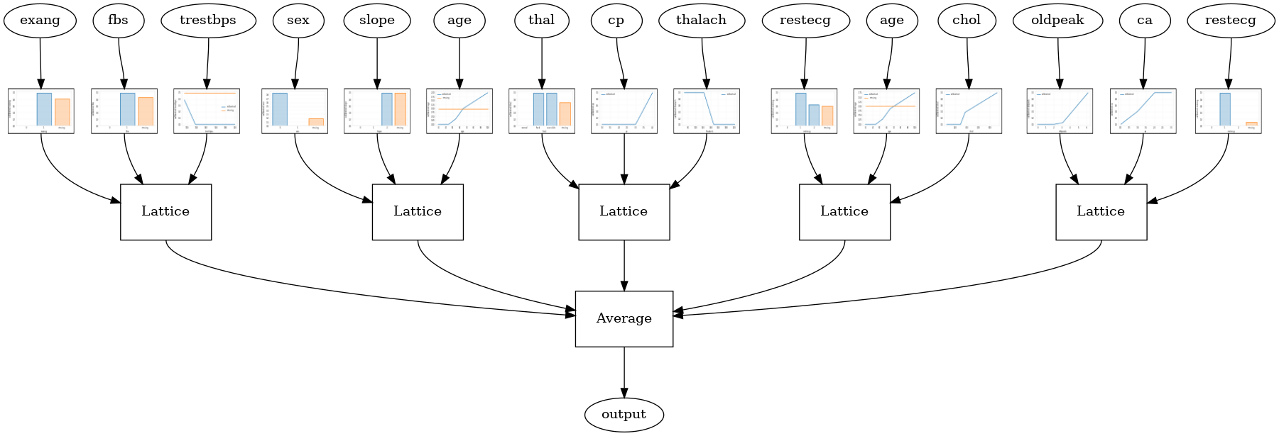
Crystals Lattice Ensemble
TFL ยังมีขั้นตอนวิธีการแก้ปัญหาคุณลักษณะการจัดเรียงที่เรียกว่า คริสตัล คริสตัล algorithm รถไฟแรกรุ่น prefitting ว่าจากจำนวนประมาณปฏิสัมพันธ์คุณลักษณะ จากนั้นจะจัดเรียงชุดสุดท้ายเพื่อให้คุณลักษณะที่มีการโต้ตอบที่ไม่เป็นเชิงเส้นมากกว่าอยู่ในโครงตาข่ายเดียวกัน
สำหรับรุ่นคริสตัลคุณยังจะต้องให้ prefitting_input_fn ที่ใช้ในการฝึกอบรมรุ่น prefitting ตามที่อธิบายไว้ข้างต้น แบบจำลองการปรับล่วงหน้าไม่จำเป็นต้องได้รับการฝึกฝนอย่างเต็มที่ ดังนั้นบางช่วงก็เพียงพอแล้ว
prefitting_input_fn = tf.compat.v1.estimator.inputs.pandas_input_fn(
    x=train_x,
    y=train_y,
    shuffle=False,
    batch_size=BATCH_SIZE,
    num_epochs=PREFITTING_NUM_EPOCHS,
    num_threads=1)
จากนั้นคุณสามารถสร้างรูปแบบคริสตัลโดยการตั้ง lattice='crystals' ในรูปแบบการตั้งค่า
# This is Crystals ensemble model with separate calibration: model output is
# the average output of separately calibrated lattices.
model_config = tfl.configs.CalibratedLatticeEnsembleConfig(
    feature_configs=feature_configs,
    lattices='crystals',
    num_lattices=5,
    lattice_rank=3)
# A CannedClassifier is constructed from the given model config.
estimator = tfl.estimators.CannedClassifier(
    feature_columns=feature_columns,
    model_config=model_config,
    feature_analysis_input_fn=feature_analysis_input_fn,
    # prefitting_input_fn is required to train the prefitting model.
    prefitting_input_fn=prefitting_input_fn,
    optimizer=tf.keras.optimizers.Adam(LEARNING_RATE),
    prefitting_optimizer=tf.keras.optimizers.Adam(LEARNING_RATE),
    config=tf.estimator.RunConfig(tf_random_seed=42))
estimator.train(input_fn=train_input_fn)
results = estimator.evaluate(input_fn=test_input_fn)
print('Crystals ensemble test AUC: {}'.format(results['auc']))
saved_model_path = estimator.export_saved_model(estimator.model_dir,
                                                serving_input_fn)
model_graph = tfl.estimators.get_model_graph(saved_model_path)
tfl.visualization.draw_model_graph(model_graph, calibrator_dpi=15)
Crystals ensemble test AUC: 0.8840851783752441
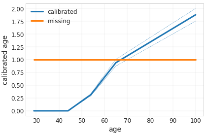
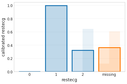
คุณสามารถพล็อตเทียบคุณลักษณะที่มีรายละเอียดเพิ่มขึ้นโดยใช้ tfl.visualization โมดูล
_ = tfl.visualization.plot_feature_calibrator(model_graph, "age")
_ = tfl.visualization.plot_feature_calibrator(model_graph, "restecg")