
| | |  ดูแหล่งที่มาบน GitHub ดูแหล่งที่มาบน GitHub | |
ภาพรวม
คุณสามารถใช้เลเยอร์ TFL Keras เพื่อสร้างแบบจำลอง Keras ที่มีความซ้ำซากจำเจและข้อจำกัดด้านรูปร่างอื่นๆ ตัวอย่างนี้สร้างและฝึกโมเดลแลตทิซที่ปรับเทียบแล้วสำหรับชุดข้อมูลหัวใจ UCI โดยใช้เลเยอร์ TFL
ในรูปแบบตาข่ายสอบเทียบแต่ละคุณลักษณะจะถูกเปลี่ยนโดย tfl.layers.PWLCalibration หรือ tfl.layers.CategoricalCalibration ชั้นและผลที่กำลังหลอมละลาย nonlinearly ใช้ tfl.layers.Lattice
ติดตั้ง
การติดตั้งแพ็คเกจ TF Lattice:
pip install -q tensorflow-lattice pydot
การนำเข้าแพ็คเกจที่จำเป็น:
import tensorflow as tf

import logging
import numpy as np
import pandas as pd
import sys
import tensorflow_lattice as tfl
from tensorflow import feature_column as fc
logging.disable(sys.maxsize)
กำลังดาวน์โหลดชุดข้อมูล UCI Statlog (หัวใจ):
# UCI Statlog (Heart) dataset.
csv_file = tf.keras.utils.get_file(
    'heart.csv', 'http://storage.googleapis.com/download.tensorflow.org/data/heart.csv')
training_data_df = pd.read_csv(csv_file).sample(
    frac=1.0, random_state=41).reset_index(drop=True)
training_data_df.head()
การตั้งค่าเริ่มต้นที่ใช้สำหรับการฝึกอบรมในคู่มือนี้:
LEARNING_RATE = 0.1
BATCH_SIZE = 128
NUM_EPOCHS = 100
โมเดล Keras ตามลำดับ
ตัวอย่างนี้สร้างโมเดล Sequential Keras และใช้เลเยอร์ TFL เท่านั้น
ชั้นตาข่ายคาดหวังว่า input[i] จะต้องอยู่ภายใน [0, lattice_sizes[i] - 1.0] ดังนั้นเราจึงจำเป็นต้องกำหนดตาข่ายขนาดไปข้างหน้าของการสอบเทียบชั้นเพื่อให้เราอย่างถูกต้องสามารถระบุช่วงการส่งออกของชั้นการสอบเทียบ
# Lattice layer expects input[i] to be within [0, lattice_sizes[i] - 1.0], so
lattice_sizes = [3, 2, 2, 2, 2, 2, 2]
เราใช้ tfl.layers.ParallelCombination ชั้นชั้นการสอบเทียบกลุ่มด้วยกันซึ่งจะต้องมีการดำเนินการในแบบคู่ขนานในการสั่งซื้อเพื่อให้สามารถสร้างรูปแบบ Sequential
combined_calibrators = tfl.layers.ParallelCombination()
เราสร้างชั้นการปรับเทียบสำหรับแต่ละคุณสมบัติและเพิ่มไปยังชั้นผสมแบบขนาน สำหรับคุณสมบัติที่เป็นตัวเลขที่เราใช้ tfl.layers.PWLCalibration และสำหรับคุณสมบัติเด็ดขาดเราใช้ tfl.layers.CategoricalCalibration
# ############### age ###############
calibrator = tfl.layers.PWLCalibration(
    # Every PWLCalibration layer must have keypoints of piecewise linear
    # function specified. Easiest way to specify them is to uniformly cover
    # entire input range by using numpy.linspace().
    input_keypoints=np.linspace(
        training_data_df['age'].min(), training_data_df['age'].max(), num=5),
    # You need to ensure that input keypoints have same dtype as layer input.
    # You can do it by setting dtype here or by providing keypoints in such
    # format which will be converted to desired tf.dtype by default.
    dtype=tf.float32,
    # Output range must correspond to expected lattice input range.
    output_min=0.0,
    output_max=lattice_sizes[0] - 1.0,
)
combined_calibrators.append(calibrator)

# ############### sex ###############
# For boolean features simply specify CategoricalCalibration layer with 2
# buckets.
calibrator = tfl.layers.CategoricalCalibration(
    num_buckets=2,
    output_min=0.0,
    output_max=lattice_sizes[1] - 1.0,
    # Initializes all outputs to (output_min + output_max) / 2.0.
    kernel_initializer='constant')
combined_calibrators.append(calibrator)

# ############### cp ###############
calibrator = tfl.layers.PWLCalibration(
    # Here instead of specifying dtype of layer we convert keypoints into
    # np.float32.
    input_keypoints=np.linspace(1, 4, num=4, dtype=np.float32),
    output_min=0.0,
    output_max=lattice_sizes[2] - 1.0,
    monotonicity='increasing',
    # You can specify TFL regularizers as a tuple ('regularizer name', l1, l2).
    kernel_regularizer=('hessian', 0.0, 1e-4))
combined_calibrators.append(calibrator)

# ############### trestbps ###############
calibrator = tfl.layers.PWLCalibration(
    # Alternatively, you might want to use quantiles as keypoints instead of
    # uniform keypoints
    input_keypoints=np.quantile(training_data_df['trestbps'],
                                np.linspace(0.0, 1.0, num=5)),
    dtype=tf.float32,
    # Together with quantile keypoints you might want to initialize piecewise
    # linear function to have 'equal_slopes' in order for output of layer
    # after initialization to preserve original distribution.
    kernel_initializer='equal_slopes',
    output_min=0.0,
    output_max=lattice_sizes[3] - 1.0,
    # You might consider clamping extreme inputs of the calibrator to output
    # bounds.
    clamp_min=True,
    clamp_max=True,
    monotonicity='increasing')
combined_calibrators.append(calibrator)

# ############### chol ###############
calibrator = tfl.layers.PWLCalibration(
    # Explicit input keypoint initialization.
    input_keypoints=[126.0, 210.0, 247.0, 286.0, 564.0],
    dtype=tf.float32,
    output_min=0.0,
    output_max=lattice_sizes[4] - 1.0,
    # Monotonicity of calibrator can be decreasing. Note that corresponding
    # lattice dimension must have INCREASING monotonicity regardless of
    # monotonicity direction of calibrator.
    monotonicity='decreasing',
    # Convexity together with decreasing monotonicity result in diminishing
    # return constraint.
    convexity='convex',
    # You can specify list of regularizers. You are not limited to TFL
    # regularizrs. Feel free to use any :)
    kernel_regularizer=[('laplacian', 0.0, 1e-4),
                        tf.keras.regularizers.l1_l2(l1=0.001)])
combined_calibrators.append(calibrator)

# ############### fbs ###############
calibrator = tfl.layers.CategoricalCalibration(
    num_buckets=2,
    output_min=0.0,
    output_max=lattice_sizes[5] - 1.0,
    # For categorical calibration layer monotonicity is specified for pairs
    # of indices of categories. Output for first category in pair will be
    # smaller than output for second category.
    #
    # Don't forget to set monotonicity of corresponding dimension of Lattice
    # layer to '1'.
    monotonicities=[(0, 1)],
    # This initializer is identical to default one('uniform'), but has fixed
    # seed in order to simplify experimentation.
    kernel_initializer=tf.keras.initializers.RandomUniform(
        minval=0.0, maxval=lattice_sizes[5] - 1.0, seed=1))
combined_calibrators.append(calibrator)

# ############### restecg ###############
calibrator = tfl.layers.CategoricalCalibration(
    num_buckets=3,
    output_min=0.0,
    output_max=lattice_sizes[6] - 1.0,
    # Categorical monotonicity can be partial order.
    monotonicities=[(0, 1), (0, 2)],
    # Categorical calibration layer supports standard Keras regularizers.
    kernel_regularizer=tf.keras.regularizers.l1_l2(l1=0.001),
    kernel_initializer='constant')
combined_calibrators.append(calibrator)
จากนั้นเราสร้างเลเยอร์ขัดแตะเพื่อหลอมรวมเอาต์พุตของเครื่องสอบเทียบแบบไม่เชิงเส้น
โปรดทราบว่าเราจำเป็นต้องระบุความซ้ำซากจำเจของโครงตาข่ายเพื่อเพิ่มขนาดที่ต้องการ องค์ประกอบที่มีทิศทางของความซ้ำซากจำเจในการสอบเทียบจะส่งผลให้ทิศทางของโมโนโทนิกจากต้นทางถึงปลายทางที่ถูกต้อง ซึ่งรวมถึงความซ้ำซากจำเจบางส่วนของชั้น CategoricalCalibration
lattice = tfl.layers.Lattice(
    lattice_sizes=lattice_sizes,
    monotonicities=[
        'increasing', 'none', 'increasing', 'increasing', 'increasing',
        'increasing', 'increasing'
    ],
    output_min=0.0,
    output_max=1.0)
จากนั้น เราสามารถสร้างแบบจำลองตามลำดับโดยใช้เครื่องสอบเทียบและเลเยอร์ขัดแตะรวมกัน
model = tf.keras.models.Sequential()
model.add(combined_calibrators)
model.add(lattice)
การฝึกอบรมทำงานเหมือนกับโมเดล Keras อื่นๆ
features = training_data_df[[
    'age', 'sex', 'cp', 'trestbps', 'chol', 'fbs', 'restecg'
]].values.astype(np.float32)
target = training_data_df[['target']].values.astype(np.float32)

model.compile(
    loss=tf.keras.losses.mean_squared_error,
    optimizer=tf.keras.optimizers.Adagrad(learning_rate=LEARNING_RATE))
model.fit(
    features,
    target,
    batch_size=BATCH_SIZE,
    epochs=NUM_EPOCHS,
    validation_split=0.2,
    shuffle=False,
    verbose=0)

model.evaluate(features, target)
10/10 [==============================] - 0s 1ms/step - loss: 0.1551
0.15506614744663239
โมเดล Keras ที่ใช้งานได้
ตัวอย่างนี้ใช้ API ที่ใช้งานได้สำหรับการสร้างแบบจำลอง Keras
เป็นที่กล่าวถึงในส่วนก่อนหน้าชั้นตาข่ายคาดหวังว่า input[i] จะต้องอยู่ภายใน [0, lattice_sizes[i] - 1.0] ดังนั้นเราจึงจำเป็นต้องกำหนดขนาดตาข่ายไปข้างหน้าของชั้นการสอบเทียบเพื่อให้เราอย่างถูกต้องสามารถระบุช่วงการส่งออกของ ชั้นสอบเทียบ
# We are going to have 2-d embedding as one of lattice inputs.
lattice_sizes = [3, 2, 2, 3, 3, 2, 2]
สำหรับแต่ละคุณลักษณะ เราจำเป็นต้องสร้างชั้นป้อนข้อมูลตามด้วยชั้นสอบเทียบ สำหรับคุณสมบัติที่เป็นตัวเลขที่เราใช้ tfl.layers.PWLCalibration และสำหรับคุณสมบัติเด็ดขาดเราใช้ tfl.layers.CategoricalCalibration
model_inputs = []
lattice_inputs = []
# ############### age ###############
age_input = tf.keras.layers.Input(shape=[1], name='age')
model_inputs.append(age_input)
age_calibrator = tfl.layers.PWLCalibration(
    # Every PWLCalibration layer must have keypoints of piecewise linear
    # function specified. Easiest way to specify them is to uniformly cover
    # entire input range by using numpy.linspace().
    input_keypoints=np.linspace(
        training_data_df['age'].min(), training_data_df['age'].max(), num=5),
    # You need to ensure that input keypoints have same dtype as layer input.
    # You can do it by setting dtype here or by providing keypoints in such
    # format which will be converted to desired tf.dtype by default.
    dtype=tf.float32,
    # Output range must correspond to expected lattice input range.
    output_min=0.0,
    output_max=lattice_sizes[0] - 1.0,
    monotonicity='increasing',
    name='age_calib',
)(
    age_input)
lattice_inputs.append(age_calibrator)

# ############### sex ###############
# For boolean features simply specify CategoricalCalibration layer with 2
# buckets.
sex_input = tf.keras.layers.Input(shape=[1], name='sex')
model_inputs.append(sex_input)
sex_calibrator = tfl.layers.CategoricalCalibration(
    num_buckets=2,
    output_min=0.0,
    output_max=lattice_sizes[1] - 1.0,
    # Initializes all outputs to (output_min + output_max) / 2.0.
    kernel_initializer='constant',
    name='sex_calib',
)(
    sex_input)
lattice_inputs.append(sex_calibrator)

# ############### cp ###############
cp_input = tf.keras.layers.Input(shape=[1], name='cp')
model_inputs.append(cp_input)
cp_calibrator = tfl.layers.PWLCalibration(
    # Here instead of specifying dtype of layer we convert keypoints into
    # np.float32.
    input_keypoints=np.linspace(1, 4, num=4, dtype=np.float32),
    output_min=0.0,
    output_max=lattice_sizes[2] - 1.0,
    monotonicity='increasing',
    # You can specify TFL regularizers as tuple ('regularizer name', l1, l2).
    kernel_regularizer=('hessian', 0.0, 1e-4),
    name='cp_calib',
)(
    cp_input)
lattice_inputs.append(cp_calibrator)

# ############### trestbps ###############
trestbps_input = tf.keras.layers.Input(shape=[1], name='trestbps')
model_inputs.append(trestbps_input)
trestbps_calibrator = tfl.layers.PWLCalibration(
    # Alternatively, you might want to use quantiles as keypoints instead of
    # uniform keypoints
    input_keypoints=np.quantile(training_data_df['trestbps'],
                                np.linspace(0.0, 1.0, num=5)),
    dtype=tf.float32,
    # Together with quantile keypoints you might want to initialize piecewise
    # linear function to have 'equal_slopes' in order for output of layer
    # after initialization to preserve original distribution.
    kernel_initializer='equal_slopes',
    output_min=0.0,
    output_max=lattice_sizes[3] - 1.0,
    # You might consider clamping extreme inputs of the calibrator to output
    # bounds.
    clamp_min=True,
    clamp_max=True,
    monotonicity='increasing',
    name='trestbps_calib',
)(
    trestbps_input)
lattice_inputs.append(trestbps_calibrator)

# ############### chol ###############
chol_input = tf.keras.layers.Input(shape=[1], name='chol')
model_inputs.append(chol_input)
chol_calibrator = tfl.layers.PWLCalibration(
    # Explicit input keypoint initialization.
    input_keypoints=[126.0, 210.0, 247.0, 286.0, 564.0],
    output_min=0.0,
    output_max=lattice_sizes[4] - 1.0,
    # Monotonicity of calibrator can be decreasing. Note that corresponding
    # lattice dimension must have INCREASING monotonicity regardless of
    # monotonicity direction of calibrator.
    monotonicity='decreasing',
    # Convexity together with decreasing monotonicity result in diminishing
    # return constraint.
    convexity='convex',
    # You can specify list of regularizers. You are not limited to TFL
    # regularizrs. Feel free to use any :)
    kernel_regularizer=[('laplacian', 0.0, 1e-4),
                        tf.keras.regularizers.l1_l2(l1=0.001)],
    name='chol_calib',
)(
    chol_input)
lattice_inputs.append(chol_calibrator)

# ############### fbs ###############
fbs_input = tf.keras.layers.Input(shape=[1], name='fbs')
model_inputs.append(fbs_input)
fbs_calibrator = tfl.layers.CategoricalCalibration(
    num_buckets=2,
    output_min=0.0,
    output_max=lattice_sizes[5] - 1.0,
    # For categorical calibration layer monotonicity is specified for pairs
    # of indices of categories. Output for first category in pair will be
    # smaller than output for second category.
    #
    # Don't forget to set monotonicity of corresponding dimension of Lattice
    # layer to '1'.
    monotonicities=[(0, 1)],
    # This initializer is identical to default one ('uniform'), but has fixed
    # seed in order to simplify experimentation.
    kernel_initializer=tf.keras.initializers.RandomUniform(
        minval=0.0, maxval=lattice_sizes[5] - 1.0, seed=1),
    name='fbs_calib',
)(
    fbs_input)
lattice_inputs.append(fbs_calibrator)

# ############### restecg ###############
restecg_input = tf.keras.layers.Input(shape=[1], name='restecg')
model_inputs.append(restecg_input)
restecg_calibrator = tfl.layers.CategoricalCalibration(
    num_buckets=3,
    output_min=0.0,
    output_max=lattice_sizes[6] - 1.0,
    # Categorical monotonicity can be partial order.
    monotonicities=[(0, 1), (0, 2)],
    # Categorical calibration layer supports standard Keras regularizers.
    kernel_regularizer=tf.keras.regularizers.l1_l2(l1=0.001),
    kernel_initializer='constant',
    name='restecg_calib',
)(
    restecg_input)
lattice_inputs.append(restecg_calibrator)
จากนั้นเราสร้างเลเยอร์ขัดแตะเพื่อหลอมรวมเอาต์พุตของเครื่องสอบเทียบแบบไม่เชิงเส้น
โปรดทราบว่าเราจำเป็นต้องระบุความซ้ำซากจำเจของโครงตาข่ายเพื่อเพิ่มขนาดที่ต้องการ องค์ประกอบที่มีทิศทางของความซ้ำซากจำเจในการสอบเทียบจะส่งผลให้ทิศทางของโมโนโทนิกจากต้นทางถึงปลายทางที่ถูกต้อง ซึ่งรวมถึง monotonicity บางส่วนของ tfl.layers.CategoricalCalibration ชั้น
lattice = tfl.layers.Lattice(
    lattice_sizes=lattice_sizes,
    monotonicities=[
        'increasing', 'none', 'increasing', 'increasing', 'increasing',
        'increasing', 'increasing'
    ],
    output_min=0.0,
    output_max=1.0,
    name='lattice',
)(
    lattice_inputs)
เพื่อเพิ่มความยืดหยุ่นให้กับโมเดล เราได้เพิ่มเลเยอร์การปรับเทียบเอาต์พุต
model_output = tfl.layers.PWLCalibration(
    input_keypoints=np.linspace(0.0, 1.0, 5),
    name='output_calib',
)(
    lattice)
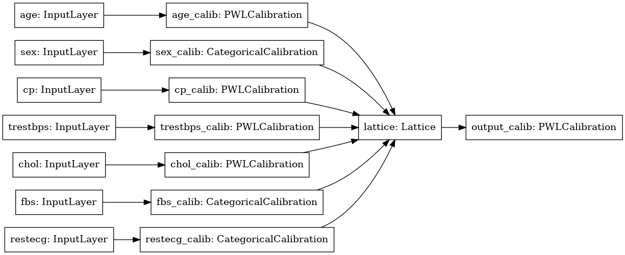
ตอนนี้เราสามารถสร้างแบบจำลองโดยใช้อินพุตและเอาต์พุต
model = tf.keras.models.Model(
    inputs=model_inputs,
    outputs=model_output)
tf.keras.utils.plot_model(model, rankdir='LR')
การฝึกอบรมทำงานเหมือนกับโมเดล Keras อื่นๆ โปรดทราบว่าด้วยการตั้งค่าของเรา คุณลักษณะการป้อนข้อมูลจะถูกส่งผ่านเป็นเมตริกซ์ที่แยกจากกัน
feature_names = ['age', 'sex', 'cp', 'trestbps', 'chol', 'fbs', 'restecg']
features = np.split(
    training_data_df[feature_names].values.astype(np.float32),
    indices_or_sections=len(feature_names),
    axis=1)
target = training_data_df[['target']].values.astype(np.float32)

model.compile(
    loss=tf.keras.losses.mean_squared_error,
    optimizer=tf.keras.optimizers.Adagrad(LEARNING_RATE))
model.fit(
    features,
    target,
    batch_size=BATCH_SIZE,
    epochs=NUM_EPOCHS,
    validation_split=0.2,
    shuffle=False,
    verbose=0)

model.evaluate(features, target)
10/10 [==============================] - 0s 1ms/step - loss: 0.1590
0.15900751948356628