
| | |  Xem nguồn trên GitHub Xem nguồn trên GitHub | |
Tổng quat
Hướng dẫn này trình bày cách thư viện TensorFlow Lattice (TFL) có thể được sử dụng để mô hình đào tạo mà cư xử có trách nhiệm, và không vi phạm một số giả định rằng là đạo đức hay công bằng. Đặc biệt, chúng tôi sẽ tập trung vào việc sử dụng hạn chế đơn điệu để tránh bị phạt không công bằng các thuộc tính nhất định. Hướng dẫn này bao gồm các cuộc biểu tình của các thí nghiệm từ giấy Deontological Đạo đức By đơn điệu chế Shape bởi Serena Wang và Maya Gupta, xuất bản tại AISTATS 2020 .
Chúng tôi sẽ sử dụng công cụ ước tính đóng hộp TFL trên tập dữ liệu công khai, nhưng lưu ý rằng mọi thứ trong hướng dẫn này cũng có thể được thực hiện với các mô hình được xây dựng từ các lớp TFL Keras.
Trước khi tiếp tục, hãy đảm bảo rằng thời gian chạy của bạn đã cài đặt tất cả các gói bắt buộc (như được nhập trong các ô mã bên dưới).
Thành lập
Cài đặt gói TF Lattice:
pip install tensorflow-lattice seaborn
Nhập các gói bắt buộc:
import tensorflow as tf

import logging
import matplotlib.pyplot as plt
import numpy as np
import os
import pandas as pd
import seaborn as sns
from sklearn.model_selection import train_test_split
import sys
import tensorflow_lattice as tfl
logging.disable(sys.maxsize)
Các giá trị mặc định được sử dụng trong hướng dẫn này:
# List of learning rate hyperparameters to try.
# For a longer list of reasonable hyperparameters, try [0.001, 0.01, 0.1].
LEARNING_RATES = [0.01]
# Default number of training epochs and batch sizes.
NUM_EPOCHS = 1000
BATCH_SIZE = 1000
# Directory containing dataset files.
DATA_DIR = 'https://raw.githubusercontent.com/serenalwang/shape_constraints_for_ethics/master'
Nghiên cứu điển hình số 1: Tuyển sinh trường luật
Trong phần đầu của hướng dẫn này, chúng tôi sẽ xem xét một nghiên cứu điển hình bằng cách sử dụng bộ dữ liệu Tuyển sinh Trường Luật từ Hội đồng Tuyển sinh Trường Luật (LSAC). Chúng tôi sẽ đào tạo một bộ phân loại để dự đoán liệu một sinh viên có vượt qua ngưỡng này hay không bằng cách sử dụng hai tính năng: điểm LSAT của sinh viên và điểm trung bình đại học.
Giả sử rằng điểm của bộ phân loại được sử dụng để hướng dẫn tuyển sinh trường luật hoặc học bổng. Theo tiêu chuẩn xã hội dựa trên thành tích, chúng tôi mong đợi rằng những sinh viên có điểm trung bình cao hơn và điểm LSAT cao hơn sẽ nhận được điểm số cao hơn từ bộ phân loại. Tuy nhiên, chúng tôi sẽ nhận thấy rằng các mô hình rất dễ vi phạm các tiêu chuẩn trực quan này và đôi khi phạt những người có điểm GPA hoặc LSAT cao hơn.
Để giải quyết vấn đề xử phạt không công bằng này, chúng ta có thể áp đặt những hạn chế đơn điệu để một mô hình không bao giờ phạt cao hơn điểm trung bình hoặc điểm LSAT cao hơn, tất cả khác nhau. Trong hướng dẫn này, chúng tôi sẽ chỉ ra cách áp đặt các ràng buộc đơn điệu đó bằng cách sử dụng TFL.
Tải dữ liệu trường luật
# Load data file.
law_file_name = 'lsac.csv'
law_file_path = os.path.join(DATA_DIR, law_file_name)
raw_law_df = pd.read_csv(law_file_path, delimiter=',')
Tập dữ liệu tiền xử lý:
# Define label column name.
LAW_LABEL = 'pass_bar'
def preprocess_law_data(input_df):
  # Drop rows with where the label or features of interest are missing.
  output_df = input_df[~input_df[LAW_LABEL].isna() & ~input_df['ugpa'].isna() &
                       (input_df['ugpa'] > 0) & ~input_df['lsat'].isna()]
  return output_df


law_df = preprocess_law_data(raw_law_df)
Chia dữ liệu thành các tập hợp đào tạo / xác nhận / kiểm tra
def split_dataset(input_df, random_state=888):
  """Splits an input dataset into train, val, and test sets."""
  train_df, test_val_df = train_test_split(
      input_df, test_size=0.3, random_state=random_state)
  val_df, test_df = train_test_split(
      test_val_df, test_size=0.66, random_state=random_state)
  return train_df, val_df, test_df


law_train_df, law_val_df, law_test_df = split_dataset(law_df)
Trực quan hóa phân phối dữ liệu
Đầu tiên chúng ta sẽ hình dung sự phân bố của dữ liệu. Chúng tôi sẽ vẽ biểu đồ điểm GPA và LSAT cho tất cả học sinh vượt qua ngưỡng này và cũng cho tất cả học sinh không vượt qua ngưỡng này.
def plot_dataset_contour(input_df, title):
  plt.rcParams['font.family'] = ['serif']
  g = sns.jointplot(
      x='ugpa',
      y='lsat',
      data=input_df,
      kind='kde',
      xlim=[1.4, 4],
      ylim=[0, 50])
  g.plot_joint(plt.scatter, c='b', s=10, linewidth=1, marker='+')
  g.ax_joint.collections[0].set_alpha(0)
  g.set_axis_labels('Undergraduate GPA', 'LSAT score', fontsize=14)
  g.fig.suptitle(title, fontsize=14)
  # Adust plot so that the title fits.
  plt.subplots_adjust(top=0.9)
  plt.show()
law_df_pos = law_df[law_df[LAW_LABEL] == 1]
plot_dataset_contour(
    law_df_pos, title='Distribution of students that passed the bar')

law_df_neg = law_df[law_df[LAW_LABEL] == 0]
plot_dataset_contour(
    law_df_neg, title='Distribution of students that failed the bar')

Đào tạo mô hình tuyến tính đã hiệu chỉnh để dự đoán việc vượt qua kỳ thi thanh
Tiếp theo, chúng tôi sẽ đào tạo một mô hình tuyến tính cỡ từ TFL để dự đoán hay không một sinh viên sẽ vượt qua quầy bar. Hai đặc điểm đầu vào sẽ là điểm LSAT và điểm trung bình ở bậc đại học, và nhãn đào tạo sẽ là liệu sinh viên có vượt qua ngưỡng hay không.
Đầu tiên chúng ta sẽ đào tạo một mô hình tuyến tính đã hiệu chỉnh mà không có bất kỳ ràng buộc nào. Sau đó, chúng tôi sẽ đào tạo một mô hình tuyến tính đã hiệu chỉnh với các ràng buộc về tính đơn điệu và quan sát sự khác biệt trong đầu ra và độ chính xác của mô hình.
Chức năng trợ giúp để đào tạo công cụ ước lượng tuyến tính đã hiệu chỉnh TFL
Các chức năng này sẽ được sử dụng cho nghiên cứu điển hình của trường luật này, cũng như nghiên cứu điển hình về tín dụng mặc định bên dưới.
def train_tfl_estimator(train_df, monotonicity, learning_rate, num_epochs,
                        batch_size, get_input_fn,
                        get_feature_columns_and_configs):
  """Trains a TFL calibrated linear estimator.

  Args:
    train_df: pandas dataframe containing training data.
    monotonicity: if 0, then no monotonicity constraints. If 1, then all
      features are constrained to be monotonically increasing.
    learning_rate: learning rate of Adam optimizer for gradient descent.
    num_epochs: number of training epochs.
    batch_size: batch size for each epoch. None means the batch size is the full
      dataset size.
    get_input_fn: function that returns the input_fn for a TF estimator.
    get_feature_columns_and_configs: function that returns TFL feature columns
      and configs.

  Returns:
    estimator: a trained TFL calibrated linear estimator.

  """
  feature_columns, feature_configs = get_feature_columns_and_configs(
      monotonicity)

  model_config = tfl.configs.CalibratedLinearConfig(
      feature_configs=feature_configs, use_bias=False)

  estimator = tfl.estimators.CannedClassifier(
      feature_columns=feature_columns,
      model_config=model_config,
      feature_analysis_input_fn=get_input_fn(input_df=train_df, num_epochs=1),
      optimizer=tf.keras.optimizers.Adam(learning_rate))

  estimator.train(
      input_fn=get_input_fn(
          input_df=train_df, num_epochs=num_epochs, batch_size=batch_size))
  return estimator


def optimize_learning_rates(
    train_df,
    val_df,
    test_df,
    monotonicity,
    learning_rates,
    num_epochs,
    batch_size,
    get_input_fn,
    get_feature_columns_and_configs,
):
  """Optimizes learning rates for TFL estimators.

  Args:
    train_df: pandas dataframe containing training data.
    val_df: pandas dataframe containing validation data.
    test_df: pandas dataframe containing test data.
    monotonicity: if 0, then no monotonicity constraints. If 1, then all
      features are constrained to be monotonically increasing.
    learning_rates: list of learning rates to try.
    num_epochs: number of training epochs.
    batch_size: batch size for each epoch. None means the batch size is the full
      dataset size.
    get_input_fn: function that returns the input_fn for a TF estimator.
    get_feature_columns_and_configs: function that returns TFL feature columns
      and configs.

  Returns:
    A single TFL estimator that achieved the best validation accuracy.
  """
  estimators = []
  train_accuracies = []
  val_accuracies = []
  test_accuracies = []
  for lr in learning_rates:
    estimator = train_tfl_estimator(
        train_df=train_df,
        monotonicity=monotonicity,
        learning_rate=lr,
        num_epochs=num_epochs,
        batch_size=batch_size,
        get_input_fn=get_input_fn,
        get_feature_columns_and_configs=get_feature_columns_and_configs)
    estimators.append(estimator)
    train_acc = estimator.evaluate(
        input_fn=get_input_fn(train_df, num_epochs=1))['accuracy']
    val_acc = estimator.evaluate(
        input_fn=get_input_fn(val_df, num_epochs=1))['accuracy']
    test_acc = estimator.evaluate(
        input_fn=get_input_fn(test_df, num_epochs=1))['accuracy']
    print('accuracies for learning rate %f: train: %f, val: %f, test: %f' %
          (lr, train_acc, val_acc, test_acc))
    train_accuracies.append(train_acc)
    val_accuracies.append(val_acc)
    test_accuracies.append(test_acc)
  max_index = val_accuracies.index(max(val_accuracies))
  return estimators[max_index]
Chức năng của người trợ giúp để định cấu hình các tính năng của tập dữ liệu trường luật
Các chức năng trợ giúp này dành riêng cho nghiên cứu trường hợp luật.
def get_input_fn_law(input_df, num_epochs, batch_size=None):
  """Gets TF input_fn for law school models."""
  return tf.compat.v1.estimator.inputs.pandas_input_fn(
      x=input_df[['ugpa', 'lsat']],
      y=input_df['pass_bar'],
      num_epochs=num_epochs,
      batch_size=batch_size or len(input_df),
      shuffle=False)


def get_feature_columns_and_configs_law(monotonicity):
  """Gets TFL feature configs for law school models."""
  feature_columns = [
      tf.feature_column.numeric_column('ugpa'),
      tf.feature_column.numeric_column('lsat'),
  ]
  feature_configs = [
      tfl.configs.FeatureConfig(
          name='ugpa',
          lattice_size=2,
          pwl_calibration_num_keypoints=20,
          monotonicity=monotonicity,
          pwl_calibration_always_monotonic=False),
      tfl.configs.FeatureConfig(
          name='lsat',
          lattice_size=2,
          pwl_calibration_num_keypoints=20,
          monotonicity=monotonicity,
          pwl_calibration_always_monotonic=False),
  ]
  return feature_columns, feature_configs
Chức năng trợ giúp để trực quan hóa kết quả đầu ra của mô hình được đào tạo
def get_predicted_probabilities(estimator, input_df, get_input_fn):
  predictions = estimator.predict(
      input_fn=get_input_fn(input_df=input_df, num_epochs=1))
  return [prediction['probabilities'][1] for prediction in predictions]


def plot_model_contour(estimator, input_df, num_keypoints=20):
  x = np.linspace(min(input_df['ugpa']), max(input_df['ugpa']), num_keypoints)
  y = np.linspace(min(input_df['lsat']), max(input_df['lsat']), num_keypoints)

  x_grid, y_grid = np.meshgrid(x, y)

  positions = np.vstack([x_grid.ravel(), y_grid.ravel()])
  plot_df = pd.DataFrame(positions.T, columns=['ugpa', 'lsat'])
  plot_df[LAW_LABEL] = np.ones(len(plot_df))
  predictions = get_predicted_probabilities(
      estimator=estimator, input_df=plot_df, get_input_fn=get_input_fn_law)
  grid_predictions = np.reshape(predictions, x_grid.shape)

  plt.rcParams['font.family'] = ['serif']
  plt.contour(
      x_grid,
      y_grid,
      grid_predictions,
      colors=('k',),
      levels=np.linspace(0, 1, 11))
  plt.contourf(
      x_grid,
      y_grid,
      grid_predictions,
      cmap=plt.cm.bone,
      levels=np.linspace(0, 1, 11))  # levels=np.linspace(0,1,8));
  plt.xticks(fontsize=20)
  plt.yticks(fontsize=20)

  cbar = plt.colorbar()
  cbar.ax.set_ylabel('Model score', fontsize=20)
  cbar.ax.tick_params(labelsize=20)

  plt.xlabel('Undergraduate GPA', fontsize=20)
  plt.ylabel('LSAT score', fontsize=20)
Đào tạo mô hình tuyến tính đã hiệu chỉnh không bị giới hạn (không đơn điệu)
nomon_linear_estimator = optimize_learning_rates(
    train_df=law_train_df,
    val_df=law_val_df,
    test_df=law_test_df,
    monotonicity=0,
    learning_rates=LEARNING_RATES,
    batch_size=BATCH_SIZE,
    num_epochs=NUM_EPOCHS,
    get_input_fn=get_input_fn_law,
    get_feature_columns_and_configs=get_feature_columns_and_configs_law)
2021-09-30 20:56:50.475180: E tensorflow/stream_executor/cuda/cuda_driver.cc:271] failed call to cuInit: CUDA_ERROR_NO_DEVICE: no CUDA-capable device is detected
accuracies for learning rate 0.010000: train: 0.949061, val: 0.945876, test: 0.951781
plot_model_contour(nomon_linear_estimator, input_df=law_df)
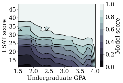
Đào tạo mô hình tuyến tính hiệu chỉnh đơn điệu
mon_linear_estimator = optimize_learning_rates(
    train_df=law_train_df,
    val_df=law_val_df,
    test_df=law_test_df,
    monotonicity=1,
    learning_rates=LEARNING_RATES,
    batch_size=BATCH_SIZE,
    num_epochs=NUM_EPOCHS,
    get_input_fn=get_input_fn_law,
    get_feature_columns_and_configs=get_feature_columns_and_configs_law)
accuracies for learning rate 0.010000: train: 0.949249, val: 0.945447, test: 0.951781
plot_model_contour(mon_linear_estimator, input_df=law_df)

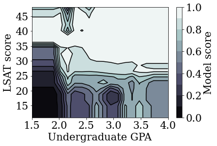
Đào tạo các mô hình không bị hạn chế khác
Chúng tôi đã chứng minh rằng các mô hình tuyến tính đã hiệu chỉnh TFL có thể được đào tạo để trở thành đơn điệu trong cả điểm LSAT và GPA mà không phải hy sinh quá nhiều về độ chính xác.
Tuy nhiên, làm thế nào để mô hình tuyến tính đã hiệu chỉnh so sánh với các loại mô hình khác, như mạng nơ ron sâu (DNN) hoặc cây tăng cường độ dốc (GBT)? Các DNN và GBT dường như có kết quả đầu ra hợp lý công bằng? Để giải quyết câu hỏi này, tiếp theo chúng tôi sẽ đào tạo DNN và GBT không bị giới hạn. Trên thực tế, chúng ta sẽ thấy rằng cả DNN và GBT đều dễ dàng vi phạm tính đơn điệu trong điểm LSAT và điểm trung bình đại học.
Đào tạo mô hình Mạng nơ ron sâu (DNN) không bị giới hạn
Kiến trúc trước đây đã được tối ưu hóa để đạt được độ chính xác xác thực cao.
feature_names = ['ugpa', 'lsat']

dnn_estimator = tf.estimator.DNNClassifier(
    feature_columns=[
        tf.feature_column.numeric_column(feature) for feature in feature_names
    ],
    hidden_units=[100, 100],
    optimizer=tf.keras.optimizers.Adam(learning_rate=0.008),
    activation_fn=tf.nn.relu)

dnn_estimator.train(
    input_fn=get_input_fn_law(
        law_train_df, batch_size=BATCH_SIZE, num_epochs=NUM_EPOCHS))
dnn_train_acc = dnn_estimator.evaluate(
    input_fn=get_input_fn_law(law_train_df, num_epochs=1))['accuracy']
dnn_val_acc = dnn_estimator.evaluate(
    input_fn=get_input_fn_law(law_val_df, num_epochs=1))['accuracy']
dnn_test_acc = dnn_estimator.evaluate(
    input_fn=get_input_fn_law(law_test_df, num_epochs=1))['accuracy']
print('accuracies for DNN: train: %f, val: %f, test: %f' %
      (dnn_train_acc, dnn_val_acc, dnn_test_acc))
accuracies for DNN: train: 0.948874, val: 0.946735, test: 0.951559
plot_model_contour(dnn_estimator, input_df=law_df)

Đào tạo mô hình Cây tăng cường Gradient (GBT) không bị giới hạn
Cấu trúc cây trước đây đã được tối ưu hóa để đạt được độ chính xác xác thực cao.
tree_estimator = tf.estimator.BoostedTreesClassifier(
    feature_columns=[
        tf.feature_column.numeric_column(feature) for feature in feature_names
    ],
    n_batches_per_layer=2,
    n_trees=20,
    max_depth=4)

tree_estimator.train(
    input_fn=get_input_fn_law(
        law_train_df, num_epochs=NUM_EPOCHS, batch_size=BATCH_SIZE))
tree_train_acc = tree_estimator.evaluate(
    input_fn=get_input_fn_law(law_train_df, num_epochs=1))['accuracy']
tree_val_acc = tree_estimator.evaluate(
    input_fn=get_input_fn_law(law_val_df, num_epochs=1))['accuracy']
tree_test_acc = tree_estimator.evaluate(
    input_fn=get_input_fn_law(law_test_df, num_epochs=1))['accuracy']
print('accuracies for GBT: train: %f, val: %f, test: %f' %
      (tree_train_acc, tree_val_acc, tree_test_acc))
accuracies for GBT: train: 0.949249, val: 0.945017, test: 0.950896
plot_model_contour(tree_estimator, input_df=law_df)
Nghiên cứu điển hình số 2: Mặc định Tín dụng
Nghiên cứu điển hình thứ hai mà chúng ta sẽ xem xét trong hướng dẫn này là dự đoán xác suất vỡ nợ tín dụng của một cá nhân. Chúng tôi sẽ sử dụng bộ dữ liệu Mặc định của Khách hàng Thẻ Tín dụng từ kho lưu trữ UCI. Dữ liệu này được thu thập từ 30.000 người dùng thẻ tín dụng Đài Loan và chứa nhãn nhị phân về việc người dùng có mặc định thanh toán trong một khoảng thời gian hay không. Các tính năng bao gồm tình trạng hôn nhân, giới tính, học vấn và thời gian người dùng chậm thanh toán các hóa đơn hiện có của họ, cho mỗi tháng từ tháng 4 đến tháng 9 năm 2005.
Như chúng ta đã làm với các nghiên cứu trường hợp đầu tiên, chúng tôi một lần nữa minh họa sử dụng hạn chế đơn điệu để tránh bị phạt không công bằng: nếu mô hình đã được sử dụng để xác định điểm tín dụng của người dùng, nó có thể cảm thấy không công bằng đối với nhiều nếu họ bị phạt vì thanh toán hóa đơn của họ sớm hơn, tất cả là như nhau. Do đó, chúng tôi áp dụng một ràng buộc đơn điệu để giữ cho mô hình không bị phạt các khoản thanh toán sớm.
Tải dữ liệu mặc định tín dụng
# Load data file.
credit_file_name = 'credit_default.csv'
credit_file_path = os.path.join(DATA_DIR, credit_file_name)
credit_df = pd.read_csv(credit_file_path, delimiter=',')
# Define label column name.
CREDIT_LABEL = 'default'
Chia dữ liệu thành các tập hợp đào tạo / xác nhận / kiểm tra
credit_train_df, credit_val_df, credit_test_df = split_dataset(credit_df)
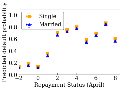
Trực quan hóa phân phối dữ liệu
Đầu tiên chúng ta sẽ hình dung sự phân bố của dữ liệu. Chúng tôi sẽ vẽ biểu đồ sai số trung bình và tiêu chuẩn của tỷ lệ mặc định quan sát được đối với những người có tình trạng hôn nhân và tình trạng trả nợ khác nhau. Tình trạng hoàn trả thể hiện số tháng mà một người phải trả sau khoản vay của họ (tính đến tháng 4 năm 2005).
def get_agg_data(df, x_col, y_col, bins=11):
  xbins = pd.cut(df[x_col], bins=bins)
  data = df[[x_col, y_col]].groupby(xbins).agg(['mean', 'sem'])
  return data


def plot_2d_means_credit(input_df, x_col, y_col, x_label, y_label):
  plt.rcParams['font.family'] = ['serif']
  _, ax = plt.subplots(nrows=1, ncols=1)
  plt.setp(ax.spines.values(), color='black', linewidth=1)
  ax.tick_params(
      direction='in', length=6, width=1, top=False, right=False, labelsize=18)
  df_single = get_agg_data(input_df[input_df['MARRIAGE'] == 1], x_col, y_col)
  df_married = get_agg_data(input_df[input_df['MARRIAGE'] == 2], x_col, y_col)
  ax.errorbar(
      df_single[(x_col, 'mean')],
      df_single[(y_col, 'mean')],
      xerr=df_single[(x_col, 'sem')],
      yerr=df_single[(y_col, 'sem')],
      color='orange',
      marker='s',
      capsize=3,
      capthick=1,
      label='Single',
      markersize=10,
      linestyle='')
  ax.errorbar(
      df_married[(x_col, 'mean')],
      df_married[(y_col, 'mean')],
      xerr=df_married[(x_col, 'sem')],
      yerr=df_married[(y_col, 'sem')],
      color='b',
      marker='^',
      capsize=3,
      capthick=1,
      label='Married',
      markersize=10,
      linestyle='')
  leg = ax.legend(loc='upper left', fontsize=18, frameon=True, numpoints=1)
  ax.set_xlabel(x_label, fontsize=18)
  ax.set_ylabel(y_label, fontsize=18)
  ax.set_ylim(0, 1.1)
  ax.set_xlim(-2, 8.5)
  ax.patch.set_facecolor('white')
  leg.get_frame().set_edgecolor('black')
  leg.get_frame().set_facecolor('white')
  leg.get_frame().set_linewidth(1)
  plt.show()
plot_2d_means_credit(credit_train_df, 'PAY_0', 'default',
                     'Repayment Status (April)', 'Observed default rate')

Đào tạo mô hình tuyến tính đã hiệu chỉnh để dự đoán tỷ lệ mặc định tín dụng
Tiếp theo, chúng tôi sẽ đào tạo một mô hình tuyến tính cỡ từ TFL để dự đoán hay không phải là người sẽ mặc định theo dạng cho mượn. Hai đặc điểm đầu vào sẽ là tình trạng hôn nhân của người đó và người đó còn bao nhiêu tháng để trả các khoản vay của họ vào tháng 4 (tình trạng trả nợ). Nhãn đào tạo sẽ là người đó có vỡ nợ hay không.
Đầu tiên chúng ta sẽ đào tạo một mô hình tuyến tính đã hiệu chỉnh mà không có bất kỳ ràng buộc nào. Sau đó, chúng tôi sẽ đào tạo một mô hình tuyến tính đã hiệu chỉnh với các ràng buộc về tính đơn điệu và quan sát sự khác biệt trong đầu ra và độ chính xác của mô hình.
Chức năng của người trợ giúp để định cấu hình các tính năng của tập dữ liệu mặc định tín dụng
Các chức năng trợ giúp này dành riêng cho nghiên cứu trường hợp mặc định tín dụng.
def get_input_fn_credit(input_df, num_epochs, batch_size=None):
  """Gets TF input_fn for credit default models."""
  return tf.compat.v1.estimator.inputs.pandas_input_fn(
      x=input_df[['MARRIAGE', 'PAY_0']],
      y=input_df['default'],
      num_epochs=num_epochs,
      batch_size=batch_size or len(input_df),
      shuffle=False)


def get_feature_columns_and_configs_credit(monotonicity):
  """Gets TFL feature configs for credit default models."""
  feature_columns = [
      tf.feature_column.numeric_column('MARRIAGE'),
      tf.feature_column.numeric_column('PAY_0'),
  ]
  feature_configs = [
      tfl.configs.FeatureConfig(
          name='MARRIAGE',
          lattice_size=2,
          pwl_calibration_num_keypoints=3,
          monotonicity=monotonicity,
          pwl_calibration_always_monotonic=False),
      tfl.configs.FeatureConfig(
          name='PAY_0',
          lattice_size=2,
          pwl_calibration_num_keypoints=10,
          monotonicity=monotonicity,
          pwl_calibration_always_monotonic=False),
  ]
  return feature_columns, feature_configs
Chức năng trợ giúp để trực quan hóa kết quả đầu ra của mô hình được đào tạo
def plot_predictions_credit(input_df,
                            estimator,
                            x_col,
                            x_label='Repayment Status (April)',
                            y_label='Predicted default probability'):
  predictions = get_predicted_probabilities(
      estimator=estimator, input_df=input_df, get_input_fn=get_input_fn_credit)
  new_df = input_df.copy()
  new_df.loc[:, 'predictions'] = predictions
  plot_2d_means_credit(new_df, x_col, 'predictions', x_label, y_label)
Đào tạo mô hình tuyến tính đã hiệu chỉnh không bị giới hạn (không đơn điệu)
nomon_linear_estimator = optimize_learning_rates(
    train_df=credit_train_df,
    val_df=credit_val_df,
    test_df=credit_test_df,
    monotonicity=0,
    learning_rates=LEARNING_RATES,
    batch_size=BATCH_SIZE,
    num_epochs=NUM_EPOCHS,
    get_input_fn=get_input_fn_credit,
    get_feature_columns_and_configs=get_feature_columns_and_configs_credit)
accuracies for learning rate 0.010000: train: 0.818762, val: 0.830065, test: 0.817172
plot_predictions_credit(credit_train_df, nomon_linear_estimator, 'PAY_0')
Đào tạo mô hình tuyến tính hiệu chỉnh đơn điệu
mon_linear_estimator = optimize_learning_rates(
    train_df=credit_train_df,
    val_df=credit_val_df,
    test_df=credit_test_df,
    monotonicity=1,
    learning_rates=LEARNING_RATES,
    batch_size=BATCH_SIZE,
    num_epochs=NUM_EPOCHS,
    get_input_fn=get_input_fn_credit,
    get_feature_columns_and_configs=get_feature_columns_and_configs_credit)
accuracies for learning rate 0.010000: train: 0.818762, val: 0.830065, test: 0.817172
plot_predictions_credit(credit_train_df, mon_linear_estimator, 'PAY_0')
