
| | |  צפה במקור ב-GitHub צפה במקור ב-GitHub | |
מדריך זה בוחן אלגוריתמים לחישוב שיפוע עבור ערכי הציפיות של מעגלים קוונטיים.
חישוב שיפוע ערך הצפי של נתון מסוים שניתן לצפות במעגל קוונטי הוא תהליך מעורב. לערכי ציפיות של ניתנים לצפייה אין את המותרות שיש לנוסחאות גרדיאנט אנליטיות שתמיד קל לרשום אותן - שלא כמו טרנספורמציות מסורתיות של למידת מכונה כמו כפל מטריצה או חיבור וקטור שיש להן נוסחאות גרדיאנט אנליטיות שקל לרשום אותן. כתוצאה מכך, ישנן שיטות שונות לחישוב שיפוע קוונטי המועילות עבור תרחישים שונים. מדריך זה משווה ומעמיד שתי סכימות בידול שונות.
להכין
pip install tensorflow==2.7.0
התקן את TensorFlow Quantum:
pip install tensorflow-quantum
# Update package resources to account for version changes.
import importlib, pkg_resources
importlib.reload(pkg_resources)
<module 'pkg_resources' from '/tmpfs/src/tf_docs_env/lib/python3.7/site-packages/pkg_resources/__init__.py'>
כעת ייבא את TensorFlow ואת התלות של המודול:
import tensorflow as tf
import tensorflow_quantum as tfq

import cirq
import sympy
import numpy as np

# visualization tools
%matplotlib inline
import matplotlib.pyplot as plt
from cirq.contrib.svg import SVGCircuit
2022-02-04 12:25:24.733670: E tensorflow/stream_executor/cuda/cuda_driver.cc:271] failed call to cuInit: CUDA_ERROR_NO_DEVICE: no CUDA-capable device is detected
1. ראשוני
בואו נהפוך את הרעיון של חישוב שיפוע עבור מעגלים קוונטיים לקצת יותר קונקרטי. נניח שיש לך מעגל עם פרמטרים כמו זה:
qubit = cirq.GridQubit(0, 0)
my_circuit = cirq.Circuit(cirq.Y(qubit)**sympy.Symbol('alpha'))
SVGCircuit(my_circuit)
findfont: Font family ['Arial'] not found. Falling back to DejaVu Sans.

יחד עם דבר שניתן לצפות בו:
pauli_x = cirq.X(qubit)
pauli_x
cirq.X(cirq.GridQubit(0, 0))
כשאתה מסתכל על האופרטור הזה אתה יודע ש- \(⟨Y(\alpha)| X | Y(\alpha)⟩ = \sin(\pi \alpha)\)
def my_expectation(op, alpha):
    """Compute ⟨Y(alpha)| `op` | Y(alpha)⟩"""
    params = {'alpha': alpha}
    sim = cirq.Simulator()
    final_state_vector = sim.simulate(my_circuit, params).final_state_vector
    return op.expectation_from_state_vector(final_state_vector, {qubit: 0}).real


my_alpha = 0.3
print("Expectation=", my_expectation(pauli_x, my_alpha))
print("Sin Formula=", np.sin(np.pi * my_alpha))
Expectation= 0.80901700258255
Sin Formula= 0.8090169943749475
ואם אתה מגדיר \(f_{1}(\alpha) = ⟨Y(\alpha)| X | Y(\alpha)⟩\) אז \(f_{1}^{'}(\alpha) = \pi \cos(\pi \alpha)\). בוא נבדוק את זה:
def my_grad(obs, alpha, eps=0.01):
    grad = 0
    f_x = my_expectation(obs, alpha)
    f_x_prime = my_expectation(obs, alpha + eps)
    return ((f_x_prime - f_x) / eps).real


print('Finite difference:', my_grad(pauli_x, my_alpha))
print('Cosine formula:   ', np.pi * np.cos(np.pi * my_alpha))
Finite difference: 1.8063604831695557
Cosine formula:    1.8465818304904567
2. הצורך במבדיל
עם מעגלים גדולים יותר, לא תמיד יהיה לך כל כך מזל שתהיה לך נוסחה שמחשבת במדויק את שיפועים של מעגל קוונטי נתון. במקרה שנוסחה פשוטה אינה מספיקה כדי לחשב את הגרדיאנט, המחלקה tfq.differentiators.Differentiator מאפשרת לך להגדיר אלגוריתמים לחישוב ההדרגות של המעגלים שלך. לדוגמה, אתה יכול ליצור מחדש את הדוגמה לעיל ב-TensorFlow Quantum (TFQ) עם:
expectation_calculation = tfq.layers.Expectation(
    differentiator=tfq.differentiators.ForwardDifference(grid_spacing=0.01))

expectation_calculation(my_circuit,
                        operators=pauli_x,
                        symbol_names=['alpha'],
                        symbol_values=[[my_alpha]])
<tf.Tensor: shape=(1, 1), dtype=float32, numpy=array([[0.80901706]], dtype=float32)>
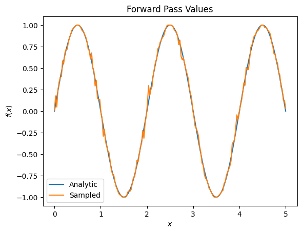
עם זאת, אם תעבור להערכת ציפיות על סמך דגימה (מה יקרה במכשיר אמיתי) הערכים יכולים להשתנות מעט. זה אומר שיש לך כעת הערכה לא מושלמת:
sampled_expectation_calculation = tfq.layers.SampledExpectation(
    differentiator=tfq.differentiators.ForwardDifference(grid_spacing=0.01))

sampled_expectation_calculation(my_circuit,
                                operators=pauli_x,
                                repetitions=500,
                                symbol_names=['alpha'],
                                symbol_values=[[my_alpha]])
<tf.Tensor: shape=(1, 1), dtype=float32, numpy=array([[0.836]], dtype=float32)>
זה יכול להוביל במהירות לבעיית דיוק רצינית בכל הנוגע לשיפועים:
# Make input_points = [batch_size, 1] array.
input_points = np.linspace(0, 5, 200)[:, np.newaxis].astype(np.float32)
exact_outputs = expectation_calculation(my_circuit,
                                        operators=pauli_x,
                                        symbol_names=['alpha'],
                                        symbol_values=input_points)
imperfect_outputs = sampled_expectation_calculation(my_circuit,
                                                    operators=pauli_x,
                                                    repetitions=500,
                                                    symbol_names=['alpha'],
                                                    symbol_values=input_points)
plt.title('Forward Pass Values')
plt.xlabel('$x$')
plt.ylabel('$f(x)$')
plt.plot(input_points, exact_outputs, label='Analytic')
plt.plot(input_points, imperfect_outputs, label='Sampled')
plt.legend()
<matplotlib.legend.Legend at 0x7ff07d556190>
# Gradients are a much different story.
values_tensor = tf.convert_to_tensor(input_points)

with tf.GradientTape() as g:
    g.watch(values_tensor)
    exact_outputs = expectation_calculation(my_circuit,
                                            operators=pauli_x,
                                            symbol_names=['alpha'],
                                            symbol_values=values_tensor)
analytic_finite_diff_gradients = g.gradient(exact_outputs, values_tensor)

with tf.GradientTape() as g:
    g.watch(values_tensor)
    imperfect_outputs = sampled_expectation_calculation(
        my_circuit,
        operators=pauli_x,
        repetitions=500,
        symbol_names=['alpha'],
        symbol_values=values_tensor)
sampled_finite_diff_gradients = g.gradient(imperfect_outputs, values_tensor)

plt.title('Gradient Values')
plt.xlabel('$x$')
plt.ylabel('$f^{\'}(x)$')
plt.plot(input_points, analytic_finite_diff_gradients, label='Analytic')
plt.plot(input_points, sampled_finite_diff_gradients, label='Sampled')
plt.legend()
<matplotlib.legend.Legend at 0x7ff07adb8dd0>
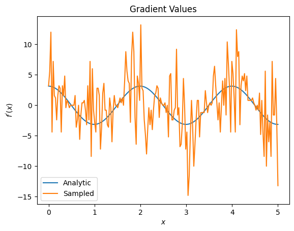
כאן אתה יכול לראות שלמרות שנוסחת ההפרש הסופי היא מהירה לחישוב הגרדיאנטים עצמם במקרה האנליטי, בכל הנוגע לשיטות מבוססות דגימה היא הייתה הרבה יותר מדי רועשת. יש להשתמש בטכניקות זהירות יותר כדי להבטיח שניתן לחשב שיפוע טוב. בשלב הבא תסתכל על טכניקה הרבה יותר איטית שלא תהיה מתאימה לחישובי שיפוע ציפיות אנליטיות, אבל היא מתפקדת הרבה יותר במקרה המבוסס על מדגם בעולם האמיתי:
# A smarter differentiation scheme.
gradient_safe_sampled_expectation = tfq.layers.SampledExpectation(
    differentiator=tfq.differentiators.ParameterShift())

with tf.GradientTape() as g:
    g.watch(values_tensor)
    imperfect_outputs = gradient_safe_sampled_expectation(
        my_circuit,
        operators=pauli_x,
        repetitions=500,
        symbol_names=['alpha'],
        symbol_values=values_tensor)

sampled_param_shift_gradients = g.gradient(imperfect_outputs, values_tensor)

plt.title('Gradient Values')
plt.xlabel('$x$')
plt.ylabel('$f^{\'}(x)$')
plt.plot(input_points, analytic_finite_diff_gradients, label='Analytic')
plt.plot(input_points, sampled_param_shift_gradients, label='Sampled')
plt.legend()
<matplotlib.legend.Legend at 0x7ff07ad9ff90>
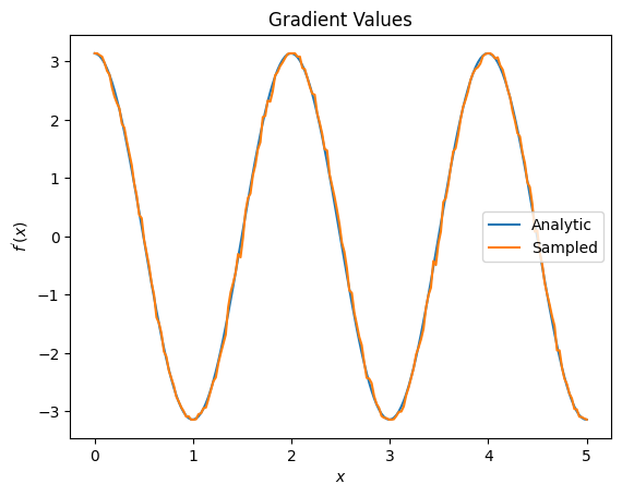
מהאמור לעיל אתה יכול לראות שמבדלים מסוימים משמשים בצורה הטובה ביותר עבור תרחישי מחקר מסוימים. באופן כללי, השיטות המבוססות על דגימות איטיות יותר, חזקות לרעש של מכשירים וכו', הן הבדלים מצוינים בעת בדיקה או יישום של אלגוריתמים בסביבה יותר "העולם האמיתי". שיטות מהירות יותר כמו הבדל סופי הן נהדרות לחישובים אנליטיים ואתה רוצה תפוקה גבוהה יותר, אבל עדיין לא עוסקים בכדאיות המכשיר של האלגוריתם שלך.
3. נצפים מרובים
הבה נציג צפייה שניה ונראה כיצד TensorFlow Quantum תומך במספר נקודות צפייה עבור מעגל בודד.
pauli_z = cirq.Z(qubit)
pauli_z
cirq.Z(cirq.GridQubit(0, 0))
אם ניתן לצפייה זה משמש עם אותו מעגל כמו קודם, אז יש לך \(f_{2}(\alpha) = ⟨Y(\alpha)| Z | Y(\alpha)⟩ = \cos(\pi \alpha)\) ו- \(f_{2}^{'}(\alpha) = -\pi \sin(\pi \alpha)\). בצע בדיקה מהירה:
test_value = 0.

print('Finite difference:', my_grad(pauli_z, test_value))
print('Sin formula:      ', -np.pi * np.sin(np.pi * test_value))
Finite difference: -0.04934072494506836
Sin formula:       -0.0
זה התאמה (קרוב מספיק).
עכשיו אם אתה מגדיר \(g(\alpha) = f_{1}(\alpha) + f_{2}(\alpha)\) אז \(g'(\alpha) = f_{1}^{'}(\alpha) + f^{'}_{2}(\alpha)\). הגדרה של יותר מצפייה אחת ב-TensorFlow Quantum לשימוש יחד עם מעגל שווה ערך להוספת מונחים נוספים ל- \(g\).
משמעות הדבר היא שהשיפוע של סמל מסוים במעגל שווה לסכום ההדרגות ביחס לכל צפייה עבור אותו סמל המוחל על אותו מעגל. זה תואם לנטילת שיפוע של TensorFlow ולהתפשטות לאחור (שם אתה נותן את סכום ההדרגות על כל הנקודות הניתנות לצפייה בתור שיפוע עבור סמל מסוים).
sum_of_outputs = tfq.layers.Expectation(
    differentiator=tfq.differentiators.ForwardDifference(grid_spacing=0.01))

sum_of_outputs(my_circuit,
               operators=[pauli_x, pauli_z],
               symbol_names=['alpha'],
               symbol_values=[[test_value]])
<tf.Tensor: shape=(1, 2), dtype=float32, numpy=array([[1.9106855e-15, 1.0000000e+00]], dtype=float32)>
כאן אתה רואה שהערך הראשון הוא הציפייה לפי פאולי X, והשני הוא הציפייה לפי פאולי Z. עכשיו כשאתה לוקח את השיפוע:
test_value_tensor = tf.convert_to_tensor([[test_value]])

with tf.GradientTape() as g:
    g.watch(test_value_tensor)
    outputs = sum_of_outputs(my_circuit,
                             operators=[pauli_x, pauli_z],
                             symbol_names=['alpha'],
                             symbol_values=test_value_tensor)

sum_of_gradients = g.gradient(outputs, test_value_tensor)

print(my_grad(pauli_x, test_value) + my_grad(pauli_z, test_value))
print(sum_of_gradients.numpy())
3.0917350202798843
[[3.0917213]]
כאן וידאת שסכום ההדרגות עבור כל נצפית הוא אכן השיפוע של \(\alpha\). התנהגות זו נתמכת על ידי כל מבחני TensorFlow Quantum וממלאת תפקיד מכריע בתאימות עם שאר TensorFlow.
4. שימוש מתקדם
כל המבדלים שקיימים בתת-מחלקה TensorFlow Quantum tfq.differentiators.Differentiator . כדי ליישם מבדל, משתמש חייב ליישם אחד משני ממשקים. התקן הוא ליישם get_gradient_circuits , אשר אומר למחלקת הבסיס אילו מעגלים למדוד כדי לקבל אומדן של השיפוע. לחלופין, אתה יכול להעמיס יתר על המידה differentiate_analytic ו- differentiate_sampled ; המחלקה tfq.differentiators.Adjoint לוקחת את המסלול הזה.
הבא משתמש ב- TensorFlow Quantum כדי ליישם את הגרדיאנט של מעגל. תשתמש בדוגמה קטנה של שינוי פרמטר.
זכור את המעגל שהגדרת למעלה, \(|\alpha⟩ = Y^{\alpha}|0⟩\). כמו קודם, אתה יכול להגדיר פונקציה כערך הצפי של מעגל זה מול ה- \(X\) הניתן לצפייה, \(f(\alpha) = ⟨\alpha|X|\alpha⟩\). באמצעות חוקי שינוי פרמטר , עבור מעגל זה, אתה יכול לגלות שהנגזרת היא
\[\frac{\partial}{\partial \alpha} f(\alpha) = \frac{\pi}{2} f\left(\alpha + \frac{1}{2}\right) - \frac{ \pi}{2} f\left(\alpha - \frac{1}{2}\right)\]
הפונקציה get_gradient_circuits מחזירה את הרכיבים של נגזרת זו.
class MyDifferentiator(tfq.differentiators.Differentiator):
    """A Toy differentiator for <Y^alpha | X |Y^alpha>."""

    def __init__(self):
        pass

    def get_gradient_circuits(self, programs, symbol_names, symbol_values):
        """Return circuits to compute gradients for given forward pass circuits.

        Every gradient on a quantum computer can be computed via measurements
        of transformed quantum circuits.  Here, you implement a custom gradient
        for a specific circuit.  For a real differentiator, you will need to
        implement this function in a more general way.  See the differentiator
        implementations in the TFQ library for examples.
        """

        # The two terms in the derivative are the same circuit...
        batch_programs = tf.stack([programs, programs], axis=1)

        # ... with shifted parameter values.
        shift = tf.constant(1/2)
        forward = symbol_values + shift
        backward = symbol_values - shift
        batch_symbol_values = tf.stack([forward, backward], axis=1)

        # Weights are the coefficients of the terms in the derivative.
        num_program_copies = tf.shape(batch_programs)[0]
        batch_weights = tf.tile(tf.constant([[[np.pi/2, -np.pi/2]]]),
                                [num_program_copies, 1, 1])

        # The index map simply says which weights go with which circuits.
        batch_mapper = tf.tile(
            tf.constant([[[0, 1]]]), [num_program_copies, 1, 1])

        return (batch_programs, symbol_names, batch_symbol_values,
                batch_weights, batch_mapper)
המחלקה הבסיסית של Differentiator משתמשת ברכיבים המוחזרים מ- get_gradient_circuits כדי לחשב את הנגזרת, כמו בנוסחת משמרת הפרמטרים שראית למעלה. כעת ניתן להשתמש במבדיל החדש הזה עם אובייקטי tfq.layer קיימים:
custom_dif = MyDifferentiator()
custom_grad_expectation = tfq.layers.Expectation(differentiator=custom_dif)

# Now let's get the gradients with finite diff.
with tf.GradientTape() as g:
    g.watch(values_tensor)
    exact_outputs = expectation_calculation(my_circuit,
                                            operators=[pauli_x],
                                            symbol_names=['alpha'],
                                            symbol_values=values_tensor)

analytic_finite_diff_gradients = g.gradient(exact_outputs, values_tensor)

# Now let's get the gradients with custom diff.
with tf.GradientTape() as g:
    g.watch(values_tensor)
    my_outputs = custom_grad_expectation(my_circuit,
                                         operators=[pauli_x],
                                         symbol_names=['alpha'],
                                         symbol_values=values_tensor)

my_gradients = g.gradient(my_outputs, values_tensor)

plt.subplot(1, 2, 1)
plt.title('Exact Gradient')
plt.plot(input_points, analytic_finite_diff_gradients.numpy())
plt.xlabel('x')
plt.ylabel('f(x)')
plt.subplot(1, 2, 2)
plt.title('My Gradient')
plt.plot(input_points, my_gradients.numpy())
plt.xlabel('x')
Text(0.5, 0, 'x')
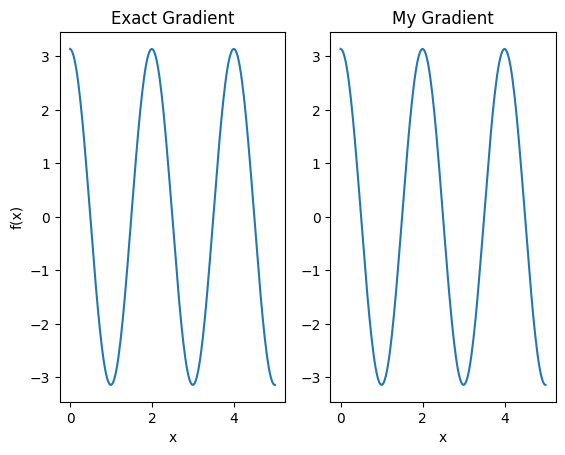
כעת ניתן להשתמש במבדיל החדש הזה כדי ליצור פעולות ניתנות להבדלה.
# Create a noisy sample based expectation op.
expectation_sampled = tfq.get_sampled_expectation_op(
    cirq.DensityMatrixSimulator(noise=cirq.depolarize(0.01)))

# Make it differentiable with your differentiator:
# Remember to refresh the differentiator before attaching the new op
custom_dif.refresh()
differentiable_op = custom_dif.generate_differentiable_op(
    sampled_op=expectation_sampled)

# Prep op inputs.
circuit_tensor = tfq.convert_to_tensor([my_circuit])
op_tensor = tfq.convert_to_tensor([[pauli_x]])
single_value = tf.convert_to_tensor([[my_alpha]])
num_samples_tensor = tf.convert_to_tensor([[5000]])

with tf.GradientTape() as g:
    g.watch(single_value)
    forward_output = differentiable_op(circuit_tensor, ['alpha'], single_value,
                                       op_tensor, num_samples_tensor)

my_gradients = g.gradient(forward_output, single_value)

print('---TFQ---')
print('Foward:  ', forward_output.numpy())
print('Gradient:', my_gradients.numpy())
print('---Original---')
print('Forward: ', my_expectation(pauli_x, my_alpha))
print('Gradient:', my_grad(pauli_x, my_alpha))
---TFQ---
Foward:   [[0.8016]]
Gradient: [[1.7932211]]
---Original---
Forward:  0.80901700258255
Gradient: 1.8063604831695557