
| |
|
 在 Github 上查看源代码 在 Github 上查看源代码 |
|
八所学校问题 (Rubin 1981) 考虑在八所学校同时进行的 SAT 辅导计划的有效性。它已经成为一个经典问题 (Bayesian Data Analysis, Stan),演示分层建模在可交换组之间共享信息的有用性。
下面的实现是 Edward 1.0 教程的改编版。
导入
import matplotlib.pyplot as plt
import numpy as np
import seaborn as sns

import tensorflow.compat.v2 as tf
import tensorflow_probability as tfp
from tensorflow_probability import distributions as tfd
import warnings

tf.enable_v2_behavior()

plt.style.use("ggplot")
warnings.filterwarnings('ignore')
数据
摘自 Bayesian Data Analysis 第 5.5 节(Gelman 等人,2013 年):
A study was performed for the Educational Testing Service to analyze the effects of special coaching programs for SAT-V (Scholastic Aptitude Test-Verbal) in each of eight high schools. The outcome variable in each study was the score on a special administration of the SAT-V, a standardized multiple choice test administered by the Educational Testing Service and used to help colleges make admissions decisions; the scores can vary between 200 and 800, with mean about 500 and standard deviation about 100. The SAT examinations are designed to be resistant to short-term efforts directed specifically toward improving performance on the test; instead they are designed to reflect knowledge acquired and abilities developed over many years of education. Nevertheless, each of the eight schools in this study considered its short-term coaching program to be very successful at increasing SAT scores. Also, there was no prior reason to believe that any of the eight programs was more effective than any other or that some were more similar in effect to each other than to any other.
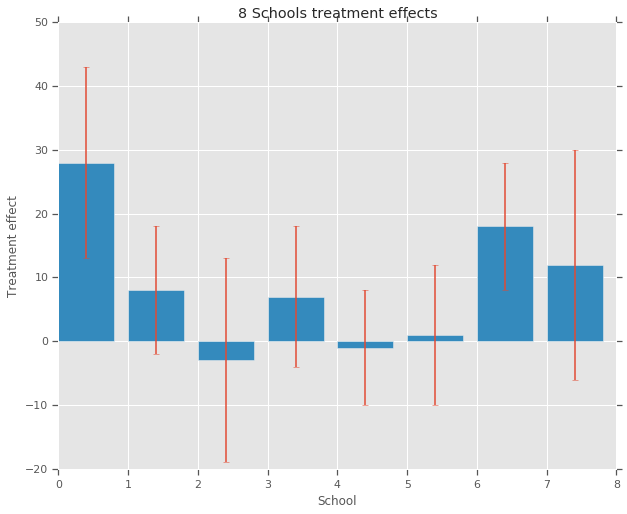
在八所学校 (\(J = 8\)) 中,每所学校都有一个估算的处理效果 \(y_j\) 和一个效果估算的标准误差 \(\sigma_j\)。我们使用 PSAT-M 和 PSAT-V 得分作为控制变量,通过对处理组进行线性回归获得研究中的处理效果。由于没有先验观念(如某些学校更加相似或更不相似,或某些辅导计划更加有效),因此我们可以认为处理效果可以互换。
num_schools = 8  # number of schools
treatment_effects = np.array(
    [28, 8, -3, 7, -1, 1, 18, 12], dtype=np.float32)  # treatment effects
treatment_stddevs = np.array(
    [15, 10, 16, 11, 9, 11, 10, 18], dtype=np.float32)  # treatment SE

fig, ax = plt.subplots()
plt.bar(range(num_schools), treatment_effects, yerr=treatment_stddevs)
plt.title("8 Schools treatment effects")
plt.xlabel("School")
plt.ylabel("Treatment effect")
fig.set_size_inches(10, 8)
plt.show()
模型
我们使用分层正态模型来捕获数据。它遵循以下生成过程,
\[ \begin{align*} \mu &\sim \text{Normal}(\text{loc}{=}0,\ \text{scale}{=}10) \ \log\tau &\sim \text{Normal}(\text{loc}{=}5,\ \text{scale}{=}1) \ \text{for } & i=1\ldots 8:\ & \theta_i \sim \text{Normal}\left(\text{loc}{=}\mu,\ \text{scale}{=}\tau \right) \ & y_i \sim \text{Normal}\left(\text{loc}{=}\theta_i,\ \text{scale}{=}\sigma_i \right) \end{align*} \]
其中 \(\mu\) 表示先验的平均处理效果,而 \(\tau\) 控制学校之间的差异。\(y_i\) 和 \(\sigma_i\) 通过观测得到。随着 \(\tau \rightarrow \infty\),该模型接近无池化模型(即,每个学校的处理效果估算可以更加独立)。随着 \(\tau \rightarrow 0\),该模型接近完整池化模型(即,所有学校的处理效果更接近组平均值 \(\mu\))。为了将标准偏差限制为正,我们从对数正态分布中绘制 \(\tau\)(这等同于从正态分布中绘制 \(log(\tau)\))。
我们按照 Diagnosing Biased Inference with Divergences 一文将上面的模型转换为等效的非中心模型:
\[ \begin{align*} \mu &\sim \text{Normal}(\text{loc}{=}0,\ \text{scale}{=}10) \ \log\tau &\sim \text{Normal}(\text{loc}{=}5,\ \text{scale}{=}1) \ \text{for } & i=1\ldots 8:\ & \theta_i' \sim \text{Normal}\left(\text{loc}{=}0,\ \text{scale}{=}1 \right) \ & \theta_i = \mu + \tau \theta_i' \ & y_i \sim \text{Normal}\left(\text{loc}{=}\theta_i,\ \text{scale}{=}\sigma_i \right) \end{align*} \]
我们将此模型具体化为 JointDistributionSequential 实例:
model = tfd.JointDistributionSequential([
  tfd.Normal(loc=0., scale=10., name="avg_effect"),  # `mu` above
  tfd.Normal(loc=5., scale=1., name="avg_stddev"),  # `log(tau)` above
  tfd.Independent(tfd.Normal(loc=tf.zeros(num_schools),
                             scale=tf.ones(num_schools),
                             name="school_effects_standard"),  # `theta_prime`
                  reinterpreted_batch_ndims=1),
  lambda school_effects_standard, avg_stddev, avg_effect: (
      tfd.Independent(tfd.Normal(loc=(avg_effect[..., tf.newaxis] +
                                      tf.exp(avg_stddev[..., tf.newaxis]) *
                                      school_effects_standard),  # `theta` above
                                 scale=treatment_stddevs),
                      name="treatment_effects",  # `y` above
                      reinterpreted_batch_ndims=1))
])

def target_log_prob_fn(avg_effect, avg_stddev, school_effects_standard):
  """Unnormalized target density as a function of states."""
  return model.log_prob((
      avg_effect, avg_stddev, school_effects_standard, treatment_effects))
贝叶斯推断
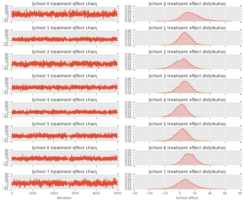
在给定数据的情况下,我们执行汉密尔顿蒙特卡洛 (HMC) 算法来计算模型参数的后验分布。
num_results = 5000
num_burnin_steps = 3000

# Improve performance by tracing the sampler using `tf.function`
# and compiling it using XLA.
@tf.function(autograph=False, jit_compile=True)
def do_sampling():
  return tfp.mcmc.sample_chain(
      num_results=num_results,
      num_burnin_steps=num_burnin_steps,
      current_state=[
          tf.zeros([], name='init_avg_effect'),
          tf.zeros([], name='init_avg_stddev'),
          tf.ones([num_schools], name='init_school_effects_standard'),
      ],
      kernel=tfp.mcmc.HamiltonianMonteCarlo(
          target_log_prob_fn=target_log_prob_fn,
          step_size=0.4,
          num_leapfrog_steps=3))

states, kernel_results = do_sampling()

avg_effect, avg_stddev, school_effects_standard = states

school_effects_samples = (
    avg_effect[:, np.newaxis] +
    np.exp(avg_stddev)[:, np.newaxis] * school_effects_standard)

num_accepted = np.sum(kernel_results.is_accepted)
print('Acceptance rate: {}'.format(num_accepted / num_results))
Acceptance rate: 0.5974
fig, axes = plt.subplots(8, 2, sharex='col', sharey='col')
fig.set_size_inches(12, 10)
for i in range(num_schools):
  axes[i][0].plot(school_effects_samples[:,i].numpy())
  axes[i][0].title.set_text("School {} treatment effect chain".format(i))
  sns.kdeplot(school_effects_samples[:,i].numpy(), ax=axes[i][1], shade=True)
  axes[i][1].title.set_text("School {} treatment effect distribution".format(i))
axes[num_schools - 1][0].set_xlabel("Iteration")
axes[num_schools - 1][1].set_xlabel("School effect")
fig.tight_layout()
plt.show()
print("E[avg_effect] = {}".format(np.mean(avg_effect)))
print("E[avg_stddev] = {}".format(np.mean(avg_stddev)))
print("E[school_effects_standard] =")
print(np.mean(school_effects_standard[:, ]))
print("E[school_effects] =")
print(np.mean(school_effects_samples[:, ], axis=0))
E[avg_effect] = 5.57183933258
E[avg_stddev] = 2.47738981247
E[school_effects_standard] =
0.08509017
E[school_effects] =
[15.0051     7.103311   2.4552586  6.2744603  1.3364682  3.1125953
 12.762501   7.743602 ]
# Compute the 95% interval for school_effects
school_effects_low = np.array([
    np.percentile(school_effects_samples[:, i], 2.5) for i in range(num_schools)
])
school_effects_med = np.array([
    np.percentile(school_effects_samples[:, i], 50) for i in range(num_schools)
])
school_effects_hi = np.array([
    np.percentile(school_effects_samples[:, i], 97.5)
    for i in range(num_schools)
])
fig, ax = plt.subplots(nrows=1, ncols=1, sharex=True)
ax.scatter(np.array(range(num_schools)), school_effects_med, color='red', s=60)
ax.scatter(
    np.array(range(num_schools)) + 0.1, treatment_effects, color='blue', s=60)

plt.plot([-0.2, 7.4], [np.mean(avg_effect),
                       np.mean(avg_effect)], 'k', linestyle='--')

ax.errorbar(
    np.array(range(8)),
    school_effects_med,
    yerr=[
        school_effects_med - school_effects_low,
        school_effects_hi - school_effects_med
    ],
    fmt='none')

ax.legend(('avg_effect', 'HMC', 'Observed effect'), fontsize=14)

plt.xlabel('School')
plt.ylabel('Treatment effect')
plt.title('HMC estimated school treatment effects vs. observed data')
fig.set_size_inches(10, 8)
plt.show()
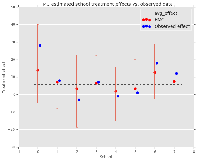
我们可以在上面观察到向 avg_effect 组的收缩。
print("Inferred posterior mean: {0:.2f}".format(
    np.mean(school_effects_samples[:,])))
print("Inferred posterior mean se: {0:.2f}".format(
    np.std(school_effects_samples[:,])))
Inferred posterior mean: 6.97
Inferred posterior mean se: 10.41
评论
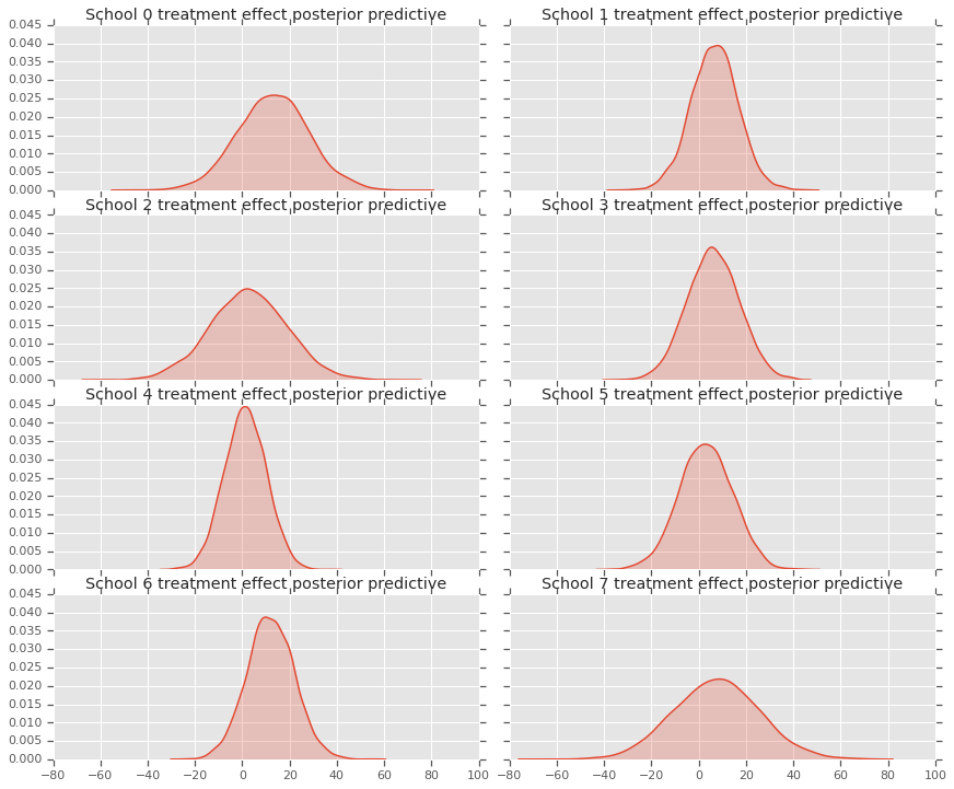
为了获得后验预测分布(即,给定观测数据 \(y\) 的情况下新数据 \(y^*\) 的模型),我们需要使用以下公式:
\[ p(y^*|y) \propto \int_\theta p(y^* | \theta)p(\theta |y)d\theta\]
我们重写模型中随机变量的值,以将它们设置为后验分布的平均值,并从该模型中采样以生成新数据 \(y^*\)。
sample_shape = [5000]

_, _, _, predictive_treatment_effects = model.sample(
    value=(tf.broadcast_to(np.mean(avg_effect, 0), sample_shape),
           tf.broadcast_to(np.mean(avg_stddev, 0), sample_shape),
           tf.broadcast_to(np.mean(school_effects_standard, 0),
                           sample_shape + [num_schools]),
           None))
fig, axes = plt.subplots(4, 2, sharex=True, sharey=True)
fig.set_size_inches(12, 10)
fig.tight_layout()
for i, ax in enumerate(axes):
  sns.kdeplot(predictive_treatment_effects[:, 2*i].numpy(),
              ax=ax[0], shade=True)
  ax[0].title.set_text(
      "School {} treatment effect posterior predictive".format(2*i))
  sns.kdeplot(predictive_treatment_effects[:, 2*i + 1].numpy(),
              ax=ax[1], shade=True)
  ax[1].title.set_text(
      "School {} treatment effect posterior predictive".format(2*i + 1))
plt.show()
# The mean predicted treatment effects for each of the eight schools.
prediction = np.mean(predictive_treatment_effects, axis=0)
我们可以看一下处理效果数据与模型后验预测值之间的残差。这些与上面的绘图相对应,该绘图显示估算效果向总体平均值收缩。
treatment_effects - prediction
array([14.905351 ,  1.2838383, -5.6966295,  0.8327627, -2.3356671,
       -2.0363257,  5.997898 ,  4.3731265], dtype=float32)
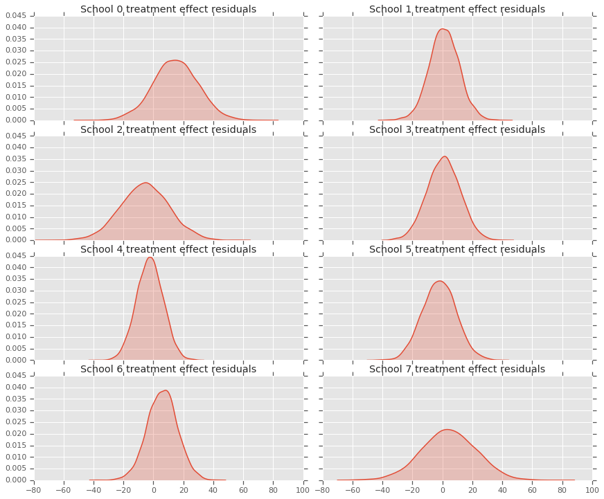
因为我们有每个学校的预测的分布,所以也可以考虑残差的分布。
residuals = treatment_effects - predictive_treatment_effects
fig, axes = plt.subplots(4, 2, sharex=True, sharey=True)
fig.set_size_inches(12, 10)
fig.tight_layout()
for i, ax in enumerate(axes):
  sns.kdeplot(residuals[:, 2*i].numpy(), ax=ax[0], shade=True)
  ax[0].title.set_text(
      "School {} treatment effect residuals".format(2*i))
  sns.kdeplot(residuals[:, 2*i + 1].numpy(), ax=ax[1], shade=True)
  ax[1].title.set_text(
      "School {} treatment effect residuals".format(2*i + 1))
plt.show()
致谢
本教程最初用 Edward 1.0 编写(源代码)。我们在此向编写和修订该版本的所有贡献者表示感谢。
参考文献
- Donald B. Rubin. Estimation in parallel randomized experiments. Journal of Educational Statistics, 6(4):377-401, 1981.
- Andrew Gelman, John Carlin, Hal Stern, David Dunson, Aki Vehtari, and Donald Rubin. Bayesian Data Analysis, Third Edition. Chapman and Hall/CRC, 2013.