TensorFlow กลับมาที่ Google I/O ในวันที่ 14 พฤษภาคม! สมัครตอนนี้

หน้านี้ได้รับการแปลโดย Cloud Translation API

โครงข่ายประสาทควอนตัม Convolutional

ดูบน TensorFlow.org

ทำงานใน Google Colab

ดูแหล่งที่มาบน GitHub

ดาวน์โหลดโน๊ตบุ๊ค

บทช่วยสอนนี้ใช้ Quantum Convolutional Neural Network (QCNN) แบบง่าย ซึ่งเป็นแอนะล็อกควอนตัมที่เสนอให้กับโครงข่ายประสาทเทียมแบบคลาสสิกซึ่ง ไม่แปรผันตามการแปล

ตัวอย่างนี้สาธิตวิธีการตรวจหาคุณสมบัติบางอย่างของแหล่งข้อมูลควอนตัม เช่น เซ็นเซอร์ควอนตัมหรือการจำลองที่ซับซ้อนจากอุปกรณ์ แหล่งข้อมูลควอนตัมเป็น สถานะคลัสเตอร์ ที่อาจมีหรือไม่มีการกระตุ้น—สิ่งที่ QCNN จะเรียนรู้ที่จะตรวจจับ (ชุดข้อมูลที่ใช้ในรายงานฉบับนี้คือการจัดประเภทเฟส SPT)

ติดตั้ง

pip install tensorflow==2.7.0

ติดตั้ง TensorFlow Quantum:

pip install tensorflow-quantum

# Update package resources to account for version changes.
import importlib, pkg_resources
importlib.reload(pkg_resources)

<module 'pkg_resources' from '/tmpfs/src/tf_docs_env/lib/python3.7/site-packages/pkg_resources/__init__.py'>

ตอนนี้นำเข้า TensorFlow และการพึ่งพาโมดูล:

import tensorflow as tf
import tensorflow_quantum as tfq

import cirq
import sympy
import numpy as np

# visualization tools
%matplotlib inline
import matplotlib.pyplot as plt
from cirq.contrib.svg import SVGCircuit

2022-02-04 12:43:45.380301: E tensorflow/stream_executor/cuda/cuda_driver.cc:271] failed call to cuInit: CUDA_ERROR_NO_DEVICE: no CUDA-capable device is detected

1. สร้าง QCNN

1.1 ประกอบวงจรในกราฟ TensorFlow

TensorFlow Quantum (TFQ) มีคลาสเลเยอร์ที่ออกแบบมาสำหรับการสร้างวงจรในกราฟ ตัวอย่างหนึ่งคือเลเยอร์ tfq.layers.AddCircuit ที่สืบทอดมาจาก tf.keras.Layer เลเยอร์นี้สามารถต่อท้ายหรือต่อท้ายชุดอินพุตของวงจร ดังแสดงในรูปต่อไปนี้

ตัวอย่างต่อไปนี้ใช้เลเยอร์นี้:

qubit = cirq.GridQubit(0, 0)

# Define some circuits.
circuit1 = cirq.Circuit(cirq.X(qubit))
circuit2 = cirq.Circuit(cirq.H(qubit))

# Convert to a tensor.
input_circuit_tensor = tfq.convert_to_tensor([circuit1, circuit2])

# Define a circuit that we want to append
y_circuit = cirq.Circuit(cirq.Y(qubit))

# Instantiate our layer
y_appender = tfq.layers.AddCircuit()

# Run our circuit tensor through the layer and save the output.
output_circuit_tensor = y_appender(input_circuit_tensor, append=y_circuit)

ตรวจสอบเทนเซอร์อินพุต:

print(tfq.from_tensor(input_circuit_tensor))

[cirq.Circuit([
     cirq.Moment(
         cirq.X(cirq.GridQubit(0, 0)),
     ),
 ])
 cirq.Circuit([
     cirq.Moment(
         cirq.H(cirq.GridQubit(0, 0)),
     ),
 ])                                   ]

และตรวจสอบเทนเซอร์เอาต์พุต:

print(tfq.from_tensor(output_circuit_tensor))

[cirq.Circuit([
     cirq.Moment(
         cirq.X(cirq.GridQubit(0, 0)),
     ),
     cirq.Moment(
         cirq.Y(cirq.GridQubit(0, 0)),
     ),
 ])
 cirq.Circuit([
     cirq.Moment(
         cirq.H(cirq.GridQubit(0, 0)),
     ),
     cirq.Moment(
         cirq.Y(cirq.GridQubit(0, 0)),
     ),
 ])                                   ]

แม้ว่าจะเป็นไปได้ที่จะเรียกใช้ตัวอย่างด้านล่างโดยไม่ต้องใช้ tfq.layers.AddCircuit แต่ก็เป็นโอกาสที่ดีที่จะทำความเข้าใจว่าฟังก์ชันที่ซับซ้อนสามารถฝังลงในกราฟการคำนวณของ TensorFlow ได้อย่างไร

1.2 ภาพรวมปัญหา

คุณจะเตรียม สถานะคลัสเตอร์ และฝึกตัวจำแนกควอนตัมเพื่อตรวจสอบว่า "ตื่นเต้น" หรือไม่ สถานะคลัสเตอร์มีความพันกันมาก แต่ไม่จำเป็นว่ายากสำหรับคอมพิวเตอร์แบบคลาสสิก เพื่อความชัดเจน นี่เป็นชุดข้อมูลที่เรียบง่ายกว่าชุดข้อมูลที่ใช้ในกระดาษ

สำหรับงานการจัดหมวดหมู่นี้ คุณจะต้องใช้สถาปัตยกรรม QCNN ที่เหมือน MERA อย่างลึกซึ้ง เนื่องจาก:

เช่นเดียวกับ QCNN สถานะของคลัสเตอร์บนวงแหวนจะไม่เปลี่ยนแปลงตามการแปล
สถานะของคลัสเตอร์จะพันกันมาก

สถาปัตยกรรมนี้ควรมีประสิทธิภาพในการลดความพัวพัน โดยได้รับการจัดประเภทโดยการอ่านควิบิตเดียว

สถานะคลัสเตอร์ "ตื่นเต้น" ถูกกำหนดให้เป็นสถานะคลัสเตอร์ที่มีเก cirq.rx ใช้กับ qubits ใดๆ Qconv และ QPool จะกล่าวถึงในภายหลังในบทช่วยสอนนี้

1.3 การสร้างบล็อคสำหรับ TensorFlow

วิธีหนึ่งในการแก้ปัญหานี้กับ TensorFlow Quantum คือการนำสิ่งต่อไปนี้ไปใช้:

อินพุตของโมเดลคือวงจรเทนเซอร์—ไม่ว่าจะเป็นวงจรว่างหรือเกท X บน qubit เฉพาะที่ระบุถึงการกระตุ้น
ส่วนประกอบควอนตัมที่เหลือของโมเดลสร้างด้วยเลเยอร์ tfq.layers.AddCircuit
สำหรับการอนุมาน จะใช้เลเยอร์ tfq.layers.PQC สิ่งนี้อ่าน \(\langle \hat{Z} \rangle\) และเปรียบเทียบกับป้ายกำกับ 1 สำหรับสถานะตื่นเต้น หรือ -1 สำหรับสถานะที่ไม่ตื่นเต้น

1.4 ข้อมูล

ก่อนสร้างแบบจำลองของคุณ คุณสามารถสร้างข้อมูลของคุณได้ ในกรณีนี้ จะเป็นการกระตุ้นสู่สถานะคลัสเตอร์ (เอกสารต้นฉบับใช้ชุดข้อมูลที่ซับซ้อนกว่า) การกระตุ้นจะแสดงด้วยประตู cirq.rx การหมุนที่ใหญ่เพียงพอจะถือเป็นการกระตุ้นและมีป้ายกำกับ 1 และการหมุนที่มีขนาดไม่มากพอจะระบุว่าเป็น -1 และถือว่าไม่ใช่การกระตุ้น

def generate_data(qubits):
    """Generate training and testing data."""
    n_rounds = 20  # Produces n_rounds * n_qubits datapoints.
    excitations = []
    labels = []
    for n in range(n_rounds):
        for bit in qubits:
            rng = np.random.uniform(-np.pi, np.pi)
            excitations.append(cirq.Circuit(cirq.rx(rng)(bit)))
            labels.append(1 if (-np.pi / 2) <= rng <= (np.pi / 2) else -1)

    split_ind = int(len(excitations) * 0.7)
    train_excitations = excitations[:split_ind]
    test_excitations = excitations[split_ind:]

    train_labels = labels[:split_ind]
    test_labels = labels[split_ind:]

    return tfq.convert_to_tensor(train_excitations), np.array(train_labels), \
        tfq.convert_to_tensor(test_excitations), np.array(test_labels)

คุณจะเห็นว่าเช่นเดียวกับการเรียนรู้ของเครื่องทั่วไป คุณสร้างชุดการฝึกอบรมและการทดสอบเพื่อใช้เปรียบเทียบโมเดล คุณสามารถดูจุดข้อมูลได้อย่างรวดเร็วด้วย:

sample_points, sample_labels, _, __ = generate_data(cirq.GridQubit.rect(1, 4))
print('Input:', tfq.from_tensor(sample_points)[0], 'Output:', sample_labels[0])
print('Input:', tfq.from_tensor(sample_points)[1], 'Output:', sample_labels[1])

Input: (0, 0): ───X^0.449─── Output: 1
Input: (0, 1): ───X^-0.74─── Output: -1

1.5 กำหนดเลเยอร์

ตอนนี้กำหนดเลเยอร์ที่แสดงในรูปด้านบนใน TensorFlow

1.5.1 สถานะคลัสเตอร์

ขั้นตอนแรกคือการกำหนด สถานะคลัสเตอร์ โดยใช้ Cirq ซึ่งเป็นเฟรมเวิร์กที่ Google จัดหาให้สำหรับการเขียนโปรแกรมวงจรควอนตัม เนื่องจากนี่เป็นส่วนคงที่ของโมเดล ให้ฝังโดยใช้ฟังก์ชัน tfq.layers.AddCircuit

def cluster_state_circuit(bits):
    """Return a cluster state on the qubits in `bits`."""
    circuit = cirq.Circuit()
    circuit.append(cirq.H.on_each(bits))
    for this_bit, next_bit in zip(bits, bits[1:] + [bits[0]]):
        circuit.append(cirq.CZ(this_bit, next_bit))
    return circuit

แสดงวงจรสถานะคลัสเตอร์สำหรับสี่เหลี่ยมผืนผ้าของ cirq.GridQubit s:

SVGCircuit(cluster_state_circuit(cirq.GridQubit.rect(1, 4)))

findfont: Font family ['Arial'] not found. Falling back to DejaVu Sans.

ตัวยึดตำแหน่ง22

svg

1.5.2 ชั้น QCNN

กำหนดเลเยอร์ที่ประกอบเป็นโมเดลโดยใช้ กระดาษ Cong และ Lukin QCNN มีข้อกำหนดเบื้องต้นบางประการ:

เมทริกซ์รวมพารามิเตอร์แบบหนึ่งและสองคิวบิตจาก กระดาษ Tucci
การดำเนินการรวมสองคิวบิตแบบกำหนดพารามิเตอร์ทั่วไป

def one_qubit_unitary(bit, symbols):
    """Make a Cirq circuit enacting a rotation of the bloch sphere about the X,
    Y and Z axis, that depends on the values in `symbols`.
    """
    return cirq.Circuit(
        cirq.X(bit)**symbols[0],
        cirq.Y(bit)**symbols[1],
        cirq.Z(bit)**symbols[2])


def two_qubit_unitary(bits, symbols):
    """Make a Cirq circuit that creates an arbitrary two qubit unitary."""
    circuit = cirq.Circuit()
    circuit += one_qubit_unitary(bits[0], symbols[0:3])
    circuit += one_qubit_unitary(bits[1], symbols[3:6])
    circuit += [cirq.ZZ(*bits)**symbols[6]]
    circuit += [cirq.YY(*bits)**symbols[7]]
    circuit += [cirq.XX(*bits)**symbols[8]]
    circuit += one_qubit_unitary(bits[0], symbols[9:12])
    circuit += one_qubit_unitary(bits[1], symbols[12:])
    return circuit


def two_qubit_pool(source_qubit, sink_qubit, symbols):
    """Make a Cirq circuit to do a parameterized 'pooling' operation, which
    attempts to reduce entanglement down from two qubits to just one."""
    pool_circuit = cirq.Circuit()
    sink_basis_selector = one_qubit_unitary(sink_qubit, symbols[0:3])
    source_basis_selector = one_qubit_unitary(source_qubit, symbols[3:6])
    pool_circuit.append(sink_basis_selector)
    pool_circuit.append(source_basis_selector)
    pool_circuit.append(cirq.CNOT(control=source_qubit, target=sink_qubit))
    pool_circuit.append(sink_basis_selector**-1)
    return pool_circuit

หากต้องการดูสิ่งที่คุณสร้าง ให้พิมพ์วงจรรวมหนึ่งควิบิต:

SVGCircuit(one_qubit_unitary(cirq.GridQubit(0, 0), sympy.symbols('x0:3')))

svg

และวงจรรวมสองควิบิต:

SVGCircuit(two_qubit_unitary(cirq.GridQubit.rect(1, 2), sympy.symbols('x0:15')))

svg

และวงจรการรวมสองควิบิต:

SVGCircuit(two_qubit_pool(*cirq.GridQubit.rect(1, 2), sympy.symbols('x0:6')))

svg

1.5.2.1 การบิดแบบควอนตัม

เช่นเดียวกับในกระดาษ Cong และ Lukin ให้นิยามคอนโวลูชัน 1D ของควอนตัมเป็นการประยุกต์ใช้การรวมพารามิเตอร์แบบสอง qubit กับทุกคู่ของ qubits ที่อยู่ติดกันด้วยการก้าวเป็นหนึ่ง

def quantum_conv_circuit(bits, symbols):
    """Quantum Convolution Layer following the above diagram.
    Return a Cirq circuit with the cascade of `two_qubit_unitary` applied
    to all pairs of qubits in `bits` as in the diagram above.
    """
    circuit = cirq.Circuit()
    for first, second in zip(bits[0::2], bits[1::2]):
        circuit += two_qubit_unitary([first, second], symbols)
    for first, second in zip(bits[1::2], bits[2::2] + [bits[0]]):
        circuit += two_qubit_unitary([first, second], symbols)
    return circuit

แสดงวงจร (แนวนอนมาก):

SVGCircuit(
    quantum_conv_circuit(cirq.GridQubit.rect(1, 8), sympy.symbols('x0:15')))

svg

1.5.2.2 การรวมควอนตัม

พูลเลเยอร์ควอนตัมพูลจาก \(N\) qubits ถึง \(\frac{N}{2}\) qubits โดยใช้พูลสองคิวบิตที่กำหนดไว้ข้างต้น

def quantum_pool_circuit(source_bits, sink_bits, symbols):
    """A layer that specifies a quantum pooling operation.
    A Quantum pool tries to learn to pool the relevant information from two
    qubits onto 1.
    """
    circuit = cirq.Circuit()
    for source, sink in zip(source_bits, sink_bits):
        circuit += two_qubit_pool(source, sink, symbols)
    return circuit

ตรวจสอบวงจรส่วนประกอบการรวม:

test_bits = cirq.GridQubit.rect(1, 8)

SVGCircuit(
    quantum_pool_circuit(test_bits[:4], test_bits[4:], sympy.symbols('x0:6')))

svg

1.6 คำจำกัดความของโมเดล

ตอนนี้ใช้เลเยอร์ที่กำหนดไว้เพื่อสร้าง CNN ควอนตัมล้วนๆ เริ่มต้นด้วยแปด qubits รวมกันเป็นหนึ่ง จากนั้นวัด \(\langle \hat{Z} \rangle\)

def create_model_circuit(qubits):
    """Create sequence of alternating convolution and pooling operators 
    which gradually shrink over time."""
    model_circuit = cirq.Circuit()
    symbols = sympy.symbols('qconv0:63')
    # Cirq uses sympy.Symbols to map learnable variables. TensorFlow Quantum
    # scans incoming circuits and replaces these with TensorFlow variables.
    model_circuit += quantum_conv_circuit(qubits, symbols[0:15])
    model_circuit += quantum_pool_circuit(qubits[:4], qubits[4:],
                                          symbols[15:21])
    model_circuit += quantum_conv_circuit(qubits[4:], symbols[21:36])
    model_circuit += quantum_pool_circuit(qubits[4:6], qubits[6:],
                                          symbols[36:42])
    model_circuit += quantum_conv_circuit(qubits[6:], symbols[42:57])
    model_circuit += quantum_pool_circuit([qubits[6]], [qubits[7]],
                                          symbols[57:63])
    return model_circuit


# Create our qubits and readout operators in Cirq.
cluster_state_bits = cirq.GridQubit.rect(1, 8)
readout_operators = cirq.Z(cluster_state_bits[-1])

# Build a sequential model enacting the logic in 1.3 of this notebook.
# Here you are making the static cluster state prep as a part of the AddCircuit and the
# "quantum datapoints" are coming in the form of excitation
excitation_input = tf.keras.Input(shape=(), dtype=tf.dtypes.string)
cluster_state = tfq.layers.AddCircuit()(
    excitation_input, prepend=cluster_state_circuit(cluster_state_bits))

quantum_model = tfq.layers.PQC(create_model_circuit(cluster_state_bits),
                               readout_operators)(cluster_state)

qcnn_model = tf.keras.Model(inputs=[excitation_input], outputs=[quantum_model])

# Show the keras plot of the model
tf.keras.utils.plot_model(qcnn_model,
                          show_shapes=True,
                          show_layer_names=False,
                          dpi=70)

png

1.7 ฝึกโมเดล

ฝึกโมเดลในแบตช์ทั้งหมดเพื่อทำให้ตัวอย่างนี้ง่ายขึ้น

# Generate some training data.
train_excitations, train_labels, test_excitations, test_labels = generate_data(
    cluster_state_bits)


# Custom accuracy metric.
@tf.function
def custom_accuracy(y_true, y_pred):
    y_true = tf.squeeze(y_true)
    y_pred = tf.map_fn(lambda x: 1.0 if x >= 0 else -1.0, y_pred)
    return tf.keras.backend.mean(tf.keras.backend.equal(y_true, y_pred))


qcnn_model.compile(optimizer=tf.keras.optimizers.Adam(learning_rate=0.02),
                   loss=tf.losses.mse,
                   metrics=[custom_accuracy])

history = qcnn_model.fit(x=train_excitations,
                         y=train_labels,
                         batch_size=16,
                         epochs=25,
                         verbose=1,
                         validation_data=(test_excitations, test_labels))

Epoch 1/25
7/7 [==============================] - 2s 176ms/step - loss: 0.8961 - custom_accuracy: 0.7143 - val_loss: 0.8012 - val_custom_accuracy: 0.7500
Epoch 2/25
7/7 [==============================] - 1s 140ms/step - loss: 0.7736 - custom_accuracy: 0.7946 - val_loss: 0.7355 - val_custom_accuracy: 0.8542
Epoch 3/25
7/7 [==============================] - 1s 138ms/step - loss: 0.7319 - custom_accuracy: 0.8393 - val_loss: 0.7045 - val_custom_accuracy: 0.8125
Epoch 4/25
7/7 [==============================] - 1s 137ms/step - loss: 0.6976 - custom_accuracy: 0.8482 - val_loss: 0.6829 - val_custom_accuracy: 0.8333
Epoch 5/25
7/7 [==============================] - 1s 143ms/step - loss: 0.6696 - custom_accuracy: 0.8750 - val_loss: 0.6749 - val_custom_accuracy: 0.7917
Epoch 6/25
7/7 [==============================] - 1s 137ms/step - loss: 0.6631 - custom_accuracy: 0.8750 - val_loss: 0.6718 - val_custom_accuracy: 0.7917
Epoch 7/25
7/7 [==============================] - 1s 135ms/step - loss: 0.6536 - custom_accuracy: 0.8929 - val_loss: 0.6638 - val_custom_accuracy: 0.8750
Epoch 8/25
7/7 [==============================] - 1s 141ms/step - loss: 0.6376 - custom_accuracy: 0.8750 - val_loss: 0.6311 - val_custom_accuracy: 0.8542
Epoch 9/25
7/7 [==============================] - 1s 137ms/step - loss: 0.6208 - custom_accuracy: 0.8750 - val_loss: 0.5995 - val_custom_accuracy: 0.8542
Epoch 10/25
7/7 [==============================] - 1s 134ms/step - loss: 0.5887 - custom_accuracy: 0.8661 - val_loss: 0.5655 - val_custom_accuracy: 0.8333
Epoch 11/25
7/7 [==============================] - 1s 144ms/step - loss: 0.5796 - custom_accuracy: 0.8482 - val_loss: 0.5681 - val_custom_accuracy: 0.8333
Epoch 12/25
7/7 [==============================] - 1s 143ms/step - loss: 0.5630 - custom_accuracy: 0.7946 - val_loss: 0.5179 - val_custom_accuracy: 0.8333
Epoch 13/25
7/7 [==============================] - 1s 137ms/step - loss: 0.5405 - custom_accuracy: 0.8304 - val_loss: 0.5003 - val_custom_accuracy: 0.8333
Epoch 14/25
7/7 [==============================] - 1s 138ms/step - loss: 0.5259 - custom_accuracy: 0.8036 - val_loss: 0.4787 - val_custom_accuracy: 0.8333
Epoch 15/25
7/7 [==============================] - 1s 137ms/step - loss: 0.5077 - custom_accuracy: 0.8482 - val_loss: 0.4741 - val_custom_accuracy: 0.8125
Epoch 16/25
7/7 [==============================] - 1s 136ms/step - loss: 0.5082 - custom_accuracy: 0.8214 - val_loss: 0.4739 - val_custom_accuracy: 0.8125
Epoch 17/25
7/7 [==============================] - 1s 137ms/step - loss: 0.5138 - custom_accuracy: 0.8214 - val_loss: 0.4859 - val_custom_accuracy: 0.8750
Epoch 18/25
7/7 [==============================] - 1s 133ms/step - loss: 0.5073 - custom_accuracy: 0.8304 - val_loss: 0.4879 - val_custom_accuracy: 0.8333
Epoch 19/25
7/7 [==============================] - 1s 138ms/step - loss: 0.5084 - custom_accuracy: 0.8304 - val_loss: 0.4745 - val_custom_accuracy: 0.8542
Epoch 20/25
7/7 [==============================] - 1s 139ms/step - loss: 0.5057 - custom_accuracy: 0.8571 - val_loss: 0.4702 - val_custom_accuracy: 0.8333
Epoch 21/25
7/7 [==============================] - 1s 135ms/step - loss: 0.4939 - custom_accuracy: 0.8304 - val_loss: 0.4734 - val_custom_accuracy: 0.8750
Epoch 22/25
7/7 [==============================] - 1s 138ms/step - loss: 0.4942 - custom_accuracy: 0.8750 - val_loss: 0.4725 - val_custom_accuracy: 0.8750
Epoch 23/25
7/7 [==============================] - 1s 140ms/step - loss: 0.4982 - custom_accuracy: 0.9107 - val_loss: 0.4695 - val_custom_accuracy: 0.8958
Epoch 24/25
7/7 [==============================] - 1s 135ms/step - loss: 0.4936 - custom_accuracy: 0.8661 - val_loss: 0.4731 - val_custom_accuracy: 0.8750
Epoch 25/25
7/7 [==============================] - 1s 136ms/step - loss: 0.4866 - custom_accuracy: 0.8571 - val_loss: 0.4631 - val_custom_accuracy: 0.8958

plt.plot(history.history['loss'][1:], label='Training')
plt.plot(history.history['val_loss'][1:], label='Validation')
plt.title('Training a Quantum CNN to Detect Excited Cluster States')
plt.xlabel('Epochs')
plt.ylabel('Loss')
plt.legend()
plt.show()

png

2. รุ่นไฮบริด

คุณไม่จำเป็นต้องเปลี่ยนจากแปด qubits เป็นหนึ่ง qubit โดยใช้ quantum convolution—คุณสามารถทำ quantum convolution หนึ่งหรือสองรอบและป้อนผลลัพธ์ลงในโครงข่ายประสาทเทียมแบบคลาสสิก ส่วนนี้สำรวจโมเดลไฮบริดควอนตัมคลาสสิก

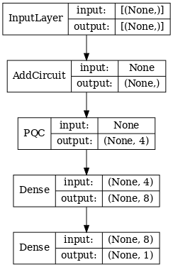
2.1 รุ่นไฮบริดที่มีตัวกรองควอนตัมตัวเดียว

ใช้การโน้มน้าวควอนตัมหนึ่งชั้น อ่านค่า \(\langle \hat{Z}_n \rangle\) ในทุกบิต ตามด้วยโครงข่ายประสาทเทียมที่เชื่อมต่ออย่างแน่นหนา

2.1.1 คำจำกัดความของโมเดล

# 1-local operators to read out
readouts = [cirq.Z(bit) for bit in cluster_state_bits[4:]]


def multi_readout_model_circuit(qubits):
    """Make a model circuit with less quantum pool and conv operations."""
    model_circuit = cirq.Circuit()
    symbols = sympy.symbols('qconv0:21')
    model_circuit += quantum_conv_circuit(qubits, symbols[0:15])
    model_circuit += quantum_pool_circuit(qubits[:4], qubits[4:],
                                          symbols[15:21])
    return model_circuit


# Build a model enacting the logic in 2.1 of this notebook.
excitation_input_dual = tf.keras.Input(shape=(), dtype=tf.dtypes.string)

cluster_state_dual = tfq.layers.AddCircuit()(
    excitation_input_dual, prepend=cluster_state_circuit(cluster_state_bits))

quantum_model_dual = tfq.layers.PQC(
    multi_readout_model_circuit(cluster_state_bits),
    readouts)(cluster_state_dual)

d1_dual = tf.keras.layers.Dense(8)(quantum_model_dual)

d2_dual = tf.keras.layers.Dense(1)(d1_dual)

hybrid_model = tf.keras.Model(inputs=[excitation_input_dual], outputs=[d2_dual])

# Display the model architecture
tf.keras.utils.plot_model(hybrid_model,
                          show_shapes=True,
                          show_layer_names=False,
                          dpi=70)

png

2.1.2 ฝึกโมเดล

hybrid_model.compile(optimizer=tf.keras.optimizers.Adam(learning_rate=0.02),
                     loss=tf.losses.mse,
                     metrics=[custom_accuracy])

hybrid_history = hybrid_model.fit(x=train_excitations,
                                  y=train_labels,
                                  batch_size=16,
                                  epochs=25,
                                  verbose=1,
                                  validation_data=(test_excitations,
                                                   test_labels))

Epoch 1/25
7/7 [==============================] - 1s 113ms/step - loss: 0.9848 - custom_accuracy: 0.5179 - val_loss: 0.9635 - val_custom_accuracy: 0.5417
Epoch 2/25
7/7 [==============================] - 1s 86ms/step - loss: 0.8095 - custom_accuracy: 0.6339 - val_loss: 0.6800 - val_custom_accuracy: 0.7083
Epoch 3/25
7/7 [==============================] - 1s 85ms/step - loss: 0.4045 - custom_accuracy: 0.9375 - val_loss: 0.3342 - val_custom_accuracy: 0.8750
Epoch 4/25
7/7 [==============================] - 1s 86ms/step - loss: 0.2308 - custom_accuracy: 0.9643 - val_loss: 0.2027 - val_custom_accuracy: 0.9792
Epoch 5/25
7/7 [==============================] - 1s 84ms/step - loss: 0.2232 - custom_accuracy: 0.9554 - val_loss: 0.1761 - val_custom_accuracy: 1.0000
Epoch 6/25
7/7 [==============================] - 1s 84ms/step - loss: 0.1760 - custom_accuracy: 0.9821 - val_loss: 0.2541 - val_custom_accuracy: 0.9167
Epoch 7/25
7/7 [==============================] - 1s 85ms/step - loss: 0.1919 - custom_accuracy: 0.9643 - val_loss: 0.1967 - val_custom_accuracy: 0.9792
Epoch 8/25
7/7 [==============================] - 1s 83ms/step - loss: 0.1892 - custom_accuracy: 0.9554 - val_loss: 0.1870 - val_custom_accuracy: 0.9792
Epoch 9/25
7/7 [==============================] - 1s 84ms/step - loss: 0.1777 - custom_accuracy: 0.9911 - val_loss: 0.2208 - val_custom_accuracy: 0.9583
Epoch 10/25
7/7 [==============================] - 1s 83ms/step - loss: 0.1728 - custom_accuracy: 0.9732 - val_loss: 0.2147 - val_custom_accuracy: 0.9583
Epoch 11/25
7/7 [==============================] - 1s 85ms/step - loss: 0.1704 - custom_accuracy: 0.9732 - val_loss: 0.1810 - val_custom_accuracy: 0.9792
Epoch 12/25
7/7 [==============================] - 1s 85ms/step - loss: 0.1739 - custom_accuracy: 0.9732 - val_loss: 0.2038 - val_custom_accuracy: 0.9792
Epoch 13/25
7/7 [==============================] - 1s 81ms/step - loss: 0.1705 - custom_accuracy: 0.9732 - val_loss: 0.1855 - val_custom_accuracy: 0.9792
Epoch 14/25
7/7 [==============================] - 1s 84ms/step - loss: 0.1788 - custom_accuracy: 0.9643 - val_loss: 0.2152 - val_custom_accuracy: 0.9583
Epoch 15/25
7/7 [==============================] - 1s 84ms/step - loss: 0.1760 - custom_accuracy: 0.9732 - val_loss: 0.1994 - val_custom_accuracy: 1.0000
Epoch 16/25
7/7 [==============================] - 1s 83ms/step - loss: 0.1737 - custom_accuracy: 0.9732 - val_loss: 0.2035 - val_custom_accuracy: 0.9792
Epoch 17/25
7/7 [==============================] - 1s 82ms/step - loss: 0.1749 - custom_accuracy: 0.9911 - val_loss: 0.1983 - val_custom_accuracy: 0.9583
Epoch 18/25
7/7 [==============================] - 1s 83ms/step - loss: 0.1875 - custom_accuracy: 0.9732 - val_loss: 0.1916 - val_custom_accuracy: 0.9583
Epoch 19/25
7/7 [==============================] - 1s 82ms/step - loss: 0.1605 - custom_accuracy: 0.9732 - val_loss: 0.1782 - val_custom_accuracy: 0.9792
Epoch 20/25
7/7 [==============================] - 1s 84ms/step - loss: 0.1668 - custom_accuracy: 0.9911 - val_loss: 0.2276 - val_custom_accuracy: 0.9583
Epoch 21/25
7/7 [==============================] - 1s 84ms/step - loss: 0.1700 - custom_accuracy: 0.9911 - val_loss: 0.2080 - val_custom_accuracy: 0.9583
Epoch 22/25
7/7 [==============================] - 1s 83ms/step - loss: 0.1621 - custom_accuracy: 0.9732 - val_loss: 0.1851 - val_custom_accuracy: 0.9375
Epoch 23/25
7/7 [==============================] - 1s 84ms/step - loss: 0.1695 - custom_accuracy: 0.9911 - val_loss: 0.1882 - val_custom_accuracy: 0.9792
Epoch 24/25
7/7 [==============================] - 1s 82ms/step - loss: 0.1583 - custom_accuracy: 0.9911 - val_loss: 0.2017 - val_custom_accuracy: 0.9583
Epoch 25/25
7/7 [==============================] - 1s 83ms/step - loss: 0.1557 - custom_accuracy: 0.9911 - val_loss: 0.1907 - val_custom_accuracy: 0.9792

plt.plot(history.history['val_custom_accuracy'], label='QCNN')
plt.plot(hybrid_history.history['val_custom_accuracy'], label='Hybrid CNN')
plt.title('Quantum vs Hybrid CNN performance')
plt.xlabel('Epochs')
plt.legend()
plt.ylabel('Validation Accuracy')
plt.show()

png

อย่างที่คุณเห็น ด้วยความช่วยเหลือแบบคลาสสิกที่เจียมเนื้อเจียมตัว โมเดลไฮบริดมักจะมาบรรจบกันเร็วกว่ารุ่นควอนตัมล้วนๆ

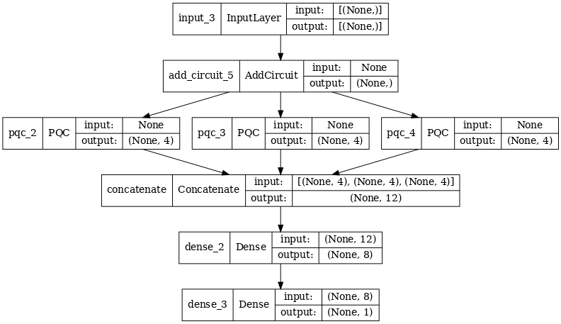
2.2 การบิดแบบไฮบริดพร้อมตัวกรองควอนตัมหลายตัว

ตอนนี้ มาลองใช้สถาปัตยกรรมที่ใช้การควอนตัมคอนโวลูชันหลายแบบและโครงข่ายประสาทเทียมแบบคลาสสิกเพื่อรวมเข้าด้วยกัน

2.2.1 คำจำกัดความของโมเดล

excitation_input_multi = tf.keras.Input(shape=(), dtype=tf.dtypes.string)

cluster_state_multi = tfq.layers.AddCircuit()(
    excitation_input_multi, prepend=cluster_state_circuit(cluster_state_bits))

# apply 3 different filters and measure expectation values

quantum_model_multi1 = tfq.layers.PQC(
    multi_readout_model_circuit(cluster_state_bits),
    readouts)(cluster_state_multi)

quantum_model_multi2 = tfq.layers.PQC(
    multi_readout_model_circuit(cluster_state_bits),
    readouts)(cluster_state_multi)

quantum_model_multi3 = tfq.layers.PQC(
    multi_readout_model_circuit(cluster_state_bits),
    readouts)(cluster_state_multi)

# concatenate outputs and feed into a small classical NN
concat_out = tf.keras.layers.concatenate(
    [quantum_model_multi1, quantum_model_multi2, quantum_model_multi3])

dense_1 = tf.keras.layers.Dense(8)(concat_out)

dense_2 = tf.keras.layers.Dense(1)(dense_1)

multi_qconv_model = tf.keras.Model(inputs=[excitation_input_multi],
                                   outputs=[dense_2])

# Display the model architecture
tf.keras.utils.plot_model(multi_qconv_model,
                          show_shapes=True,
                          show_layer_names=True,
                          dpi=70)

png

2.2.2 ฝึกโมเดล

multi_qconv_model.compile(
    optimizer=tf.keras.optimizers.Adam(learning_rate=0.02),
    loss=tf.losses.mse,
    metrics=[custom_accuracy])

multi_qconv_history = multi_qconv_model.fit(x=train_excitations,
                                            y=train_labels,
                                            batch_size=16,
                                            epochs=25,
                                            verbose=1,
                                            validation_data=(test_excitations,
                                                             test_labels))

Epoch 1/25
7/7 [==============================] - 2s 143ms/step - loss: 0.9425 - custom_accuracy: 0.6429 - val_loss: 0.8120 - val_custom_accuracy: 0.7083
Epoch 2/25
7/7 [==============================] - 1s 109ms/step - loss: 0.5778 - custom_accuracy: 0.7946 - val_loss: 0.5920 - val_custom_accuracy: 0.7500
Epoch 3/25
7/7 [==============================] - 1s 103ms/step - loss: 0.4954 - custom_accuracy: 0.9018 - val_loss: 0.4568 - val_custom_accuracy: 0.7708
Epoch 4/25
7/7 [==============================] - 1s 95ms/step - loss: 0.2855 - custom_accuracy: 0.9196 - val_loss: 0.2792 - val_custom_accuracy: 0.9375
Epoch 5/25
7/7 [==============================] - 1s 93ms/step - loss: 0.1902 - custom_accuracy: 0.9821 - val_loss: 0.2212 - val_custom_accuracy: 0.9375
Epoch 6/25
7/7 [==============================] - 1s 94ms/step - loss: 0.1685 - custom_accuracy: 0.9821 - val_loss: 0.2341 - val_custom_accuracy: 0.9583
Epoch 7/25
7/7 [==============================] - 1s 104ms/step - loss: 0.1671 - custom_accuracy: 0.9911 - val_loss: 0.2062 - val_custom_accuracy: 0.9792
Epoch 8/25
7/7 [==============================] - 1s 97ms/step - loss: 0.1511 - custom_accuracy: 0.9821 - val_loss: 0.2096 - val_custom_accuracy: 0.9792
Epoch 9/25
7/7 [==============================] - 1s 96ms/step - loss: 0.1432 - custom_accuracy: 0.9911 - val_loss: 0.2330 - val_custom_accuracy: 0.9375
Epoch 10/25
7/7 [==============================] - 1s 92ms/step - loss: 0.1668 - custom_accuracy: 0.9821 - val_loss: 0.2344 - val_custom_accuracy: 0.9583
Epoch 11/25
7/7 [==============================] - 1s 106ms/step - loss: 0.1893 - custom_accuracy: 0.9732 - val_loss: 0.2148 - val_custom_accuracy: 0.9583
Epoch 12/25
7/7 [==============================] - 1s 104ms/step - loss: 0.1857 - custom_accuracy: 0.9732 - val_loss: 0.2739 - val_custom_accuracy: 0.9583
Epoch 13/25
7/7 [==============================] - 1s 106ms/step - loss: 0.1748 - custom_accuracy: 0.9732 - val_loss: 0.2366 - val_custom_accuracy: 0.9583
Epoch 14/25
7/7 [==============================] - 1s 103ms/step - loss: 0.1515 - custom_accuracy: 0.9821 - val_loss: 0.2012 - val_custom_accuracy: 0.9583
Epoch 15/25
7/7 [==============================] - 1s 100ms/step - loss: 0.1552 - custom_accuracy: 0.9911 - val_loss: 0.2404 - val_custom_accuracy: 0.9375
Epoch 16/25
7/7 [==============================] - 1s 97ms/step - loss: 0.1572 - custom_accuracy: 0.9911 - val_loss: 0.2779 - val_custom_accuracy: 0.9375
Epoch 17/25
7/7 [==============================] - 1s 100ms/step - loss: 0.1546 - custom_accuracy: 0.9821 - val_loss: 0.2104 - val_custom_accuracy: 0.9583
Epoch 18/25
7/7 [==============================] - 1s 102ms/step - loss: 0.1418 - custom_accuracy: 0.9911 - val_loss: 0.2647 - val_custom_accuracy: 0.9583
Epoch 19/25
7/7 [==============================] - 1s 98ms/step - loss: 0.1590 - custom_accuracy: 0.9732 - val_loss: 0.2154 - val_custom_accuracy: 0.9583
Epoch 20/25
7/7 [==============================] - 1s 104ms/step - loss: 0.1363 - custom_accuracy: 1.0000 - val_loss: 0.2470 - val_custom_accuracy: 0.9375
Epoch 21/25
7/7 [==============================] - 1s 100ms/step - loss: 0.1442 - custom_accuracy: 0.9821 - val_loss: 0.2383 - val_custom_accuracy: 0.9375
Epoch 22/25
7/7 [==============================] - 1s 99ms/step - loss: 0.1415 - custom_accuracy: 0.9911 - val_loss: 0.2324 - val_custom_accuracy: 0.9583
Epoch 23/25
7/7 [==============================] - 1s 97ms/step - loss: 0.1424 - custom_accuracy: 0.9821 - val_loss: 0.2188 - val_custom_accuracy: 0.9583
Epoch 24/25
7/7 [==============================] - 1s 100ms/step - loss: 0.1417 - custom_accuracy: 0.9821 - val_loss: 0.2340 - val_custom_accuracy: 0.9375
Epoch 25/25
7/7 [==============================] - 1s 103ms/step - loss: 0.1471 - custom_accuracy: 0.9732 - val_loss: 0.2252 - val_custom_accuracy: 0.9583

plt.plot(history.history['val_custom_accuracy'][:25], label='QCNN')
plt.plot(hybrid_history.history['val_custom_accuracy'][:25], label='Hybrid CNN')
plt.plot(multi_qconv_history.history['val_custom_accuracy'][:25],
         label='Hybrid CNN \n Multiple Quantum Filters')
plt.title('Quantum vs Hybrid CNN performance')
plt.xlabel('Epochs')
plt.legend()
plt.ylabel('Validation Accuracy')
plt.show()

png