
| | |  Wyświetl źródło na GitHub Wyświetl źródło na GitHub | |
Przegląd
Premade Modele są szybkie i łatwe sposoby tworzenia TFL tf.keras.model instancje dla typowych przypadków użycia. Ten przewodnik przedstawia kroki potrzebne do skonstruowania gotowego modelu TFL i przeszkolenia/przetestowania go.
Ustawiać
Instalowanie pakietu TF Lattice:
pip install tensorflow-lattice pydot
Importowanie wymaganych pakietów:
import tensorflow as tf

import copy
import logging
import numpy as np
import pandas as pd
import sys
import tensorflow_lattice as tfl
logging.disable(sys.maxsize)
Ustawianie wartości domyślnych używanych do szkolenia w tym przewodniku:
LEARNING_RATE = 0.01
BATCH_SIZE = 128
NUM_EPOCHS = 500
PREFITTING_NUM_EPOCHS = 10
Pobieranie zbioru danych UCI Statlog (Heart):
heart_csv_file = tf.keras.utils.get_file(
    'heart.csv',
    'http://storage.googleapis.com/download.tensorflow.org/data/heart.csv')
heart_df = pd.read_csv(heart_csv_file)
thal_vocab_list = ['normal', 'fixed', 'reversible']
heart_df['thal'] = heart_df['thal'].map(
    {v: i for i, v in enumerate(thal_vocab_list)})
heart_df = heart_df.astype(float)

heart_train_size = int(len(heart_df) * 0.8)
heart_train_dict = dict(heart_df[:heart_train_size])
heart_test_dict = dict(heart_df[heart_train_size:])

# This ordering of input features should match the feature configs. If no
# feature config relies explicitly on the data (i.e. all are 'quantiles'),
# then you can construct the feature_names list by simply iterating over each
# feature config and extracting it's name.
feature_names = [
    'age', 'sex', 'cp', 'chol', 'fbs', 'trestbps', 'thalach', 'restecg',
    'exang', 'oldpeak', 'slope', 'ca', 'thal'
]

# Since we have some features that manually construct their input keypoints,
# we need an index mapping of the feature names.
feature_name_indices = {name: index for index, name in enumerate(feature_names)}

label_name = 'target'
heart_train_xs = [
    heart_train_dict[feature_name] for feature_name in feature_names
]
heart_test_xs = [heart_test_dict[feature_name] for feature_name in feature_names]
heart_train_ys = heart_train_dict[label_name]
heart_test_ys = heart_test_dict[label_name]
Downloading data from http://storage.googleapis.com/download.tensorflow.org/data/heart.csv
16384/13273 [=====================================] - 0s 0us/step
24576/13273 [=======================================================] - 0s 0us/step
Konfiguracje funkcji
Funkcja kalibracji i konfiguracji per-feature są ustawiane za pomocą tfl.configs.FeatureConfig . Konfiguracje funkcji zawiera ograniczenia monotoniczności, uregulowania per-funkcji (patrz tfl.configs.RegularizerConfig ) i rozmiary kratowe dla modeli sieciowych.
Pamiętaj, że musimy w pełni określić konfigurację funkcji dla każdej funkcji, którą nasz model ma rozpoznawać. W przeciwnym razie model nie będzie miał możliwości dowiedzenia się, że taka cecha istnieje.
Definiowanie naszych konfiguracji funkcji
Teraz, gdy możemy obliczyć nasze kwantyle, definiujemy konfigurację funkcji dla każdej funkcji, którą nasz model ma przyjąć jako dane wejściowe.
# Features:
# - age
# - sex
# - cp        chest pain type (4 values)
# - trestbps  resting blood pressure
# - chol      serum cholestoral in mg/dl
# - fbs       fasting blood sugar > 120 mg/dl
# - restecg   resting electrocardiographic results (values 0,1,2)
# - thalach   maximum heart rate achieved
# - exang     exercise induced angina
# - oldpeak   ST depression induced by exercise relative to rest
# - slope     the slope of the peak exercise ST segment
# - ca        number of major vessels (0-3) colored by flourosopy
# - thal      normal; fixed defect; reversable defect
#
# Feature configs are used to specify how each feature is calibrated and used.
heart_feature_configs = [
    tfl.configs.FeatureConfig(
        name='age',
        lattice_size=3,
        monotonicity='increasing',
        # We must set the keypoints manually.
        pwl_calibration_num_keypoints=5,
        pwl_calibration_input_keypoints='quantiles',
        pwl_calibration_clip_max=100,
        # Per feature regularization.
        regularizer_configs=[
            tfl.configs.RegularizerConfig(name='calib_wrinkle', l2=0.1),
        ],
    ),
    tfl.configs.FeatureConfig(
        name='sex',
        num_buckets=2,
    ),
    tfl.configs.FeatureConfig(
        name='cp',
        monotonicity='increasing',
        # Keypoints that are uniformly spaced.
        pwl_calibration_num_keypoints=4,
        pwl_calibration_input_keypoints=np.linspace(
            np.min(heart_train_xs[feature_name_indices['cp']]),
            np.max(heart_train_xs[feature_name_indices['cp']]),
            num=4),
    ),
    tfl.configs.FeatureConfig(
        name='chol',
        monotonicity='increasing',
        # Explicit input keypoints initialization.
        pwl_calibration_input_keypoints=[126.0, 210.0, 247.0, 286.0, 564.0],
        # Calibration can be forced to span the full output range by clamping.
        pwl_calibration_clamp_min=True,
        pwl_calibration_clamp_max=True,
        # Per feature regularization.
        regularizer_configs=[
            tfl.configs.RegularizerConfig(name='calib_hessian', l2=1e-4),
        ],
    ),
    tfl.configs.FeatureConfig(
        name='fbs',
        # Partial monotonicity: output(0) <= output(1)
        monotonicity=[(0, 1)],
        num_buckets=2,
    ),
    tfl.configs.FeatureConfig(
        name='trestbps',
        monotonicity='decreasing',
        pwl_calibration_num_keypoints=5,
        pwl_calibration_input_keypoints='quantiles',
    ),
    tfl.configs.FeatureConfig(
        name='thalach',
        monotonicity='decreasing',
        pwl_calibration_num_keypoints=5,
        pwl_calibration_input_keypoints='quantiles',
    ),
    tfl.configs.FeatureConfig(
        name='restecg',
        # Partial monotonicity: output(0) <= output(1), output(0) <= output(2)
        monotonicity=[(0, 1), (0, 2)],
        num_buckets=3,
    ),
    tfl.configs.FeatureConfig(
        name='exang',
        # Partial monotonicity: output(0) <= output(1)
        monotonicity=[(0, 1)],
        num_buckets=2,
    ),
    tfl.configs.FeatureConfig(
        name='oldpeak',
        monotonicity='increasing',
        pwl_calibration_num_keypoints=5,
        pwl_calibration_input_keypoints='quantiles',
    ),
    tfl.configs.FeatureConfig(
        name='slope',
        # Partial monotonicity: output(0) <= output(1), output(1) <= output(2)
        monotonicity=[(0, 1), (1, 2)],
        num_buckets=3,
    ),
    tfl.configs.FeatureConfig(
        name='ca',
        monotonicity='increasing',
        pwl_calibration_num_keypoints=4,
        pwl_calibration_input_keypoints='quantiles',
    ),
    tfl.configs.FeatureConfig(
        name='thal',
        # Partial monotonicity:
        # output(normal) <= output(fixed)
        # output(normal) <= output(reversible)
        monotonicity=[('normal', 'fixed'), ('normal', 'reversible')],
        num_buckets=3,
        # We must specify the vocabulary list in order to later set the
        # monotonicities since we used names and not indices.
        vocabulary_list=thal_vocab_list,
    ),
]
Ustaw monotoniczność i kluczowe punkty
Następnie musimy upewnić się, że prawidłowo ustawiliśmy monotoniczność dla funkcji, w których użyliśmy niestandardowego słownictwa (takiego jak „thal” powyżej).
tfl.premade_lib.set_categorical_monotonicities(heart_feature_configs)
Na koniec możemy uzupełnić nasze konfiguracje funkcji, obliczając i ustawiając punkty kluczowe.
feature_keypoints = tfl.premade_lib.compute_feature_keypoints(
    feature_configs=heart_feature_configs, features=heart_train_dict)
tfl.premade_lib.set_feature_keypoints(
    feature_configs=heart_feature_configs,
    feature_keypoints=feature_keypoints,
    add_missing_feature_configs=False)
Skalibrowany model liniowy
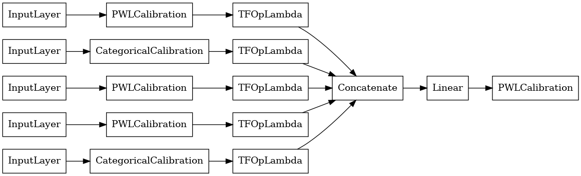
Skonstruować model predefiniowanych TFL najpierw budować konfiguracji modelu z tfl.configs . Kalibrowany model liniowy zbudowany jest przy użyciu tfl.configs.CalibratedLinearConfig . Stosuje kalibrację odcinkowo liniową i kategoryczną dla cech wejściowych, a następnie kombinację liniową i opcjonalną wyjściową kalibrację odcinkowo-liniową. Podczas korzystania z kalibracji wyjściowej lub gdy określone są granice wyjściowe, warstwa liniowa zastosuje uśrednienie ważone na skalibrowanych danych wejściowych.
Ten przykład tworzy skalibrowany model liniowy na pierwszych 5 obiektach.
# Model config defines the model structure for the premade model.
linear_model_config = tfl.configs.CalibratedLinearConfig(
    feature_configs=heart_feature_configs[:5],
    use_bias=True,
    output_calibration=True,
    output_calibration_num_keypoints=10,
    # We initialize the output to [-2.0, 2.0] since we'll be using logits.
    output_initialization=np.linspace(-2.0, 2.0, num=10),
    regularizer_configs=[
        # Regularizer for the output calibrator.
        tfl.configs.RegularizerConfig(name='output_calib_hessian', l2=1e-4),
    ])
# A CalibratedLinear premade model constructed from the given model config.
linear_model = tfl.premade.CalibratedLinear(linear_model_config)
# Let's plot our model.
tf.keras.utils.plot_model(linear_model, show_layer_names=False, rankdir='LR')
2022-01-14 12:36:31.295751: E tensorflow/stream_executor/cuda/cuda_driver.cc:271] failed call to cuInit: CUDA_ERROR_NO_DEVICE: no CUDA-capable device is detected
Teraz, jak w przypadku każdego innego tf.keras.Model , możemy skompilować i dopasować model do naszych danych.
linear_model.compile(
    loss=tf.keras.losses.BinaryCrossentropy(from_logits=True),
    metrics=[tf.keras.metrics.AUC(from_logits=True)],
    optimizer=tf.keras.optimizers.Adam(LEARNING_RATE))
linear_model.fit(
    heart_train_xs[:5],
    heart_train_ys,
    epochs=NUM_EPOCHS,
    batch_size=BATCH_SIZE,
    verbose=False)
<keras.callbacks.History at 0x7fe4385f0290>
Po wytrenowaniu naszego modelu, możemy go ocenić na naszym zestawie testowym.
print('Test Set Evaluation...')
print(linear_model.evaluate(heart_test_xs[:5], heart_test_ys))
Test Set Evaluation...
2/2 [==============================] - 0s 3ms/step - loss: 0.4728 - auc: 0.8252
[0.47278329730033875, 0.8251879215240479]
Skalibrowany model kraty
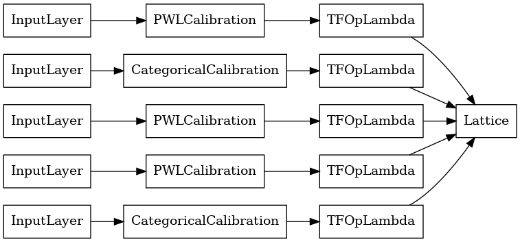
Kalibrowany kraty model jest wykonana przy użyciu tfl.configs.CalibratedLatticeConfig . Skalibrowany model sieci stosuje kalibrację odcinkowo liniową i kategoryczną na cechach wejściowych, a następnie model sieciowy i opcjonalną kalibrację odcinkowo liniową wyjściową.
Ten przykład tworzy skalibrowany model sieci na pierwszych 5 cechach.
# This is a calibrated lattice model: inputs are calibrated, then combined
# non-linearly using a lattice layer.
lattice_model_config = tfl.configs.CalibratedLatticeConfig(
    feature_configs=heart_feature_configs[:5],
    # We initialize the output to [-2.0, 2.0] since we'll be using logits.
    output_initialization=[-2.0, 2.0],
    regularizer_configs=[
        # Torsion regularizer applied to the lattice to make it more linear.
        tfl.configs.RegularizerConfig(name='torsion', l2=1e-2),
        # Globally defined calibration regularizer is applied to all features.
        tfl.configs.RegularizerConfig(name='calib_hessian', l2=1e-2),
    ])
# A CalibratedLattice premade model constructed from the given model config.
lattice_model = tfl.premade.CalibratedLattice(lattice_model_config)
# Let's plot our model.
tf.keras.utils.plot_model(lattice_model, show_layer_names=False, rankdir='LR')
Tak jak poprzednio, kompilujemy, dopasowujemy i oceniamy nasz model.
lattice_model.compile(
    loss=tf.keras.losses.BinaryCrossentropy(from_logits=True),
    metrics=[tf.keras.metrics.AUC(from_logits=True)],
    optimizer=tf.keras.optimizers.Adam(LEARNING_RATE))
lattice_model.fit(
    heart_train_xs[:5],
    heart_train_ys,
    epochs=NUM_EPOCHS,
    batch_size=BATCH_SIZE,
    verbose=False)
print('Test Set Evaluation...')
print(lattice_model.evaluate(heart_test_xs[:5], heart_test_ys))
Test Set Evaluation...
2/2 [==============================] - 1s 3ms/step - loss: 0.4709 - auc_1: 0.8302
[0.4709009826183319, 0.8302004933357239]
Skalibrowany model zespołu kratowego
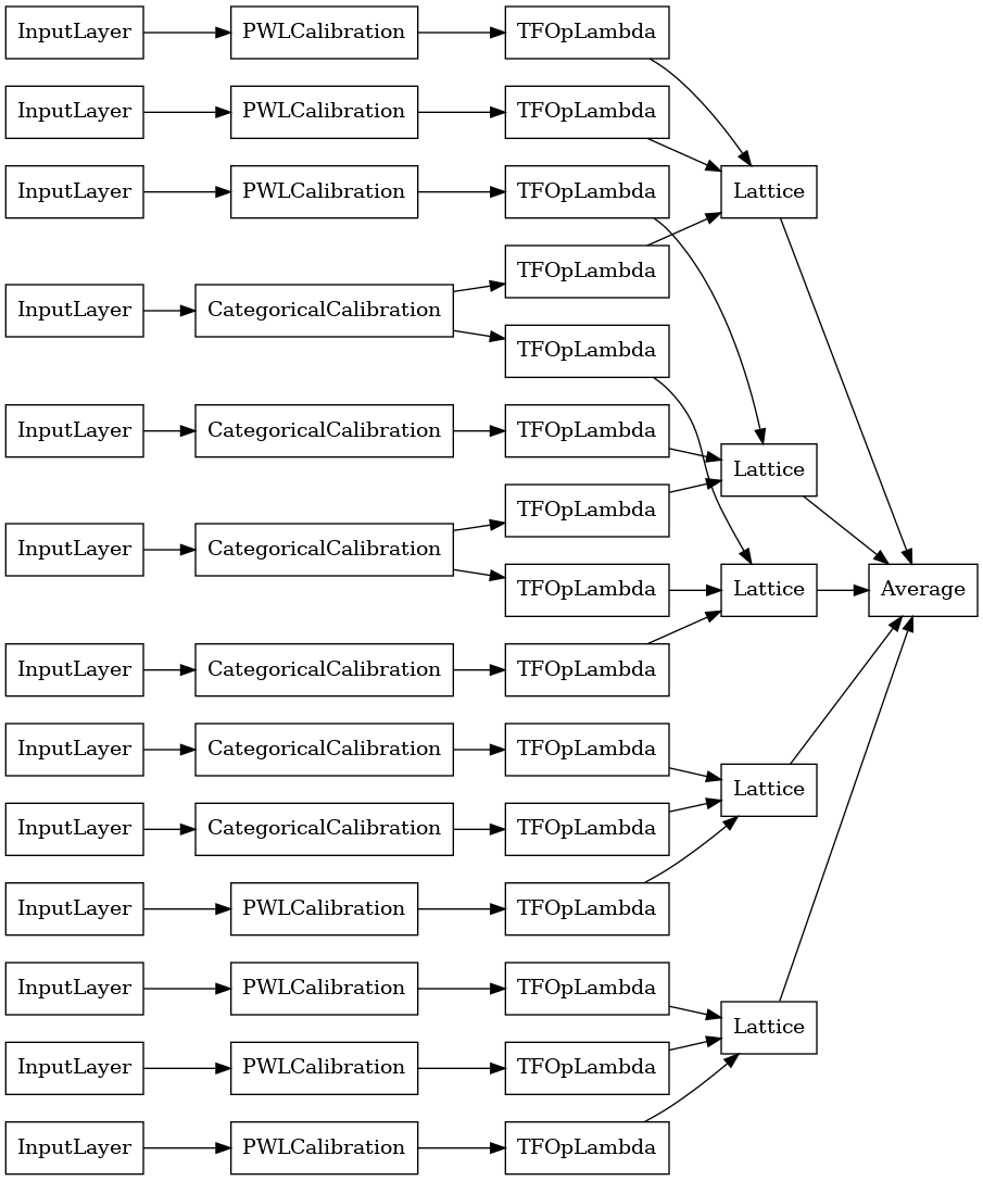
Gdy liczba funkcji jest duża, można użyć modelu zespołowego, który tworzy wiele mniejszych sieci dla podzbiorów funkcji i uśrednia ich wyniki zamiast tworzyć tylko jedną ogromną sieć. Muzycy modele kratowe są skonstruowane przy użyciu tfl.configs.CalibratedLatticeEnsembleConfig . Skalibrowany model sieciowy stosuje kalibrację odcinkowo liniową i kategoryczną na obiekcie wejściowym, a następnie zespół modeli sieci i opcjonalną kalibrację odcinkowo liniową wyjściową.
Jawna inicjalizacja zespołu kratowego
Jeśli już wiesz, które podzbiory funkcji chcesz wprowadzić do sieci, możesz jawnie ustawić sieci za pomocą nazw funkcji. Ten przykład tworzy skalibrowany model zespołu kratowego z 5 kratami i 3 elementami na kratę.
# This is a calibrated lattice ensemble model: inputs are calibrated, then
# combined non-linearly and averaged using multiple lattice layers.
explicit_ensemble_model_config = tfl.configs.CalibratedLatticeEnsembleConfig(
    feature_configs=heart_feature_configs,
    lattices=[['trestbps', 'chol', 'ca'], ['fbs', 'restecg', 'thal'],
              ['fbs', 'cp', 'oldpeak'], ['exang', 'slope', 'thalach'],
              ['restecg', 'age', 'sex']],
    num_lattices=5,
    lattice_rank=3,
    # We initialize the output to [-2.0, 2.0] since we'll be using logits.
    output_initialization=[-2.0, 2.0])
# A CalibratedLatticeEnsemble premade model constructed from the given
# model config.
explicit_ensemble_model = tfl.premade.CalibratedLatticeEnsemble(
    explicit_ensemble_model_config)
# Let's plot our model.
tf.keras.utils.plot_model(
    explicit_ensemble_model, show_layer_names=False, rankdir='LR')
Tak jak poprzednio, kompilujemy, dopasowujemy i oceniamy nasz model.
explicit_ensemble_model.compile(
    loss=tf.keras.losses.BinaryCrossentropy(from_logits=True),
    metrics=[tf.keras.metrics.AUC(from_logits=True)],
    optimizer=tf.keras.optimizers.Adam(LEARNING_RATE))
explicit_ensemble_model.fit(
    heart_train_xs,
    heart_train_ys,
    epochs=NUM_EPOCHS,
    batch_size=BATCH_SIZE,
    verbose=False)
print('Test Set Evaluation...')
print(explicit_ensemble_model.evaluate(heart_test_xs, heart_test_ys))
Test Set Evaluation...
2/2 [==============================] - 1s 4ms/step - loss: 0.3768 - auc_2: 0.8954
[0.3768467903137207, 0.895363450050354]
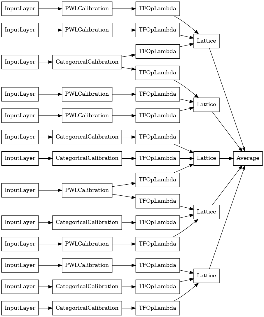
Losowy zespół kratowy
Jeśli nie masz pewności, które podzbiory funkcji wprowadzić do sieci, inną opcją jest użycie losowych podzbiorów funkcji dla każdej sieci. Ten przykład tworzy skalibrowany model zespołu kratowego z 5 kratami i 3 elementami na kratę.
# This is a calibrated lattice ensemble model: inputs are calibrated, then
# combined non-linearly and averaged using multiple lattice layers.
random_ensemble_model_config = tfl.configs.CalibratedLatticeEnsembleConfig(
    feature_configs=heart_feature_configs,
    lattices='random',
    num_lattices=5,
    lattice_rank=3,
    # We initialize the output to [-2.0, 2.0] since we'll be using logits.
    output_initialization=[-2.0, 2.0],
    random_seed=42)
# Now we must set the random lattice structure and construct the model.
tfl.premade_lib.set_random_lattice_ensemble(random_ensemble_model_config)
# A CalibratedLatticeEnsemble premade model constructed from the given
# model config.
random_ensemble_model = tfl.premade.CalibratedLatticeEnsemble(
    random_ensemble_model_config)
# Let's plot our model.
tf.keras.utils.plot_model(
    random_ensemble_model, show_layer_names=False, rankdir='LR')
Tak jak poprzednio, kompilujemy, dopasowujemy i oceniamy nasz model.
random_ensemble_model.compile(
    loss=tf.keras.losses.BinaryCrossentropy(from_logits=True),
    metrics=[tf.keras.metrics.AUC(from_logits=True)],
    optimizer=tf.keras.optimizers.Adam(LEARNING_RATE))
random_ensemble_model.fit(
    heart_train_xs,
    heart_train_ys,
    epochs=NUM_EPOCHS,
    batch_size=BATCH_SIZE,
    verbose=False)
print('Test Set Evaluation...')
print(random_ensemble_model.evaluate(heart_test_xs, heart_test_ys))
Test Set Evaluation...
2/2 [==============================] - 1s 4ms/step - loss: 0.3739 - auc_3: 0.8997
[0.3739270567893982, 0.8997493982315063]
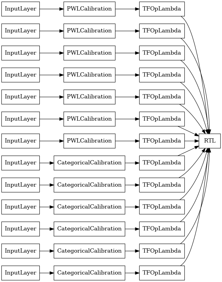
RTL Layer Random Lattice Ensemble
Podczas korzystania przypadkowy zespół kraty, można określić, że model użyć pojedynczego tfl.layers.RTL warstwę. Zauważmy, że tfl.layers.RTL obsługuje tylko ograniczenia monotoniczności i muszą mieć ten sam rozmiar siatki dla wszystkich funkcji i nie uregulowania per-feature. Należy pamiętać, że stosując tfl.layers.RTL warstwę pozwala skalować do znacznie większych niż przy użyciu oddzielnych zespołów tfl.layers.Lattice instancji.
Ten przykład tworzy skalibrowany model zespołu kratowego z 5 kratami i 3 elementami na kratę.
# Make sure our feature configs have the same lattice size, no per-feature
# regularization, and only monotonicity constraints.
rtl_layer_feature_configs = copy.deepcopy(heart_feature_configs)
for feature_config in rtl_layer_feature_configs:
  feature_config.lattice_size = 2
  feature_config.unimodality = 'none'
  feature_config.reflects_trust_in = None
  feature_config.dominates = None
  feature_config.regularizer_configs = None
# This is a calibrated lattice ensemble model: inputs are calibrated, then
# combined non-linearly and averaged using multiple lattice layers.
rtl_layer_ensemble_model_config = tfl.configs.CalibratedLatticeEnsembleConfig(
    feature_configs=rtl_layer_feature_configs,
    lattices='rtl_layer',
    num_lattices=5,
    lattice_rank=3,
    # We initialize the output to [-2.0, 2.0] since we'll be using logits.
    output_initialization=[-2.0, 2.0],
    random_seed=42)
# A CalibratedLatticeEnsemble premade model constructed from the given
# model config. Note that we do not have to specify the lattices by calling
# a helper function (like before with random) because the RTL Layer will take
# care of that for us.
rtl_layer_ensemble_model = tfl.premade.CalibratedLatticeEnsemble(
    rtl_layer_ensemble_model_config)
# Let's plot our model.
tf.keras.utils.plot_model(
    rtl_layer_ensemble_model, show_layer_names=False, rankdir='LR')
Tak jak poprzednio, kompilujemy, dopasowujemy i oceniamy nasz model.
rtl_layer_ensemble_model.compile(
    loss=tf.keras.losses.BinaryCrossentropy(from_logits=True),
    metrics=[tf.keras.metrics.AUC(from_logits=True)],
    optimizer=tf.keras.optimizers.Adam(LEARNING_RATE))
rtl_layer_ensemble_model.fit(
    heart_train_xs,
    heart_train_ys,
    epochs=NUM_EPOCHS,
    batch_size=BATCH_SIZE,
    verbose=False)
print('Test Set Evaluation...')
print(rtl_layer_ensemble_model.evaluate(heart_test_xs, heart_test_ys))
Test Set Evaluation...
2/2 [==============================] - 0s 3ms/step - loss: 0.3614 - auc_4: 0.9079
[0.36142951250076294, 0.9078947305679321]
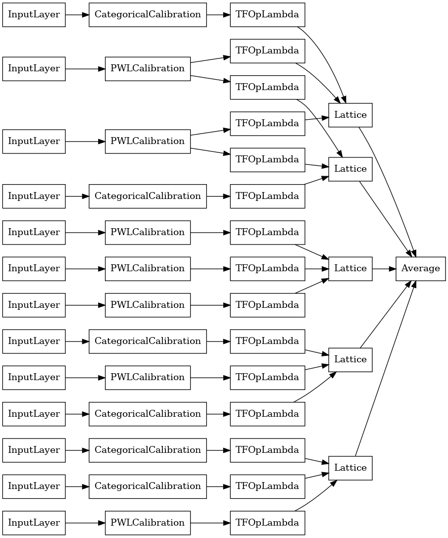
Kryształowy zespół kratowy
Premade zapewnia również algorytm heurystyczny aranżacji funkcja o nazwie Crystals . Aby użyć algorytmu Crystals, najpierw trenujemy model wstępnego dopasowania, który szacuje interakcje między cechami w parach. Następnie układamy ostateczny zespół w taki sposób, aby obiekty o bardziej nieliniowych interakcjach znajdowały się w tych samych sieciach.
Biblioteka Premade oferuje funkcje pomocnicze do konstruowania wstępnie dopasowanej konfiguracji modelu i wyodrębniania struktury kryształów. Zauważ, że model wstępnego dopasowania nie musi być w pełni wyszkolony, więc kilka epok powinno wystarczyć.
Ten przykład tworzy skalibrowany model zespołu kratowego z 5 kratami i 3 elementami na kratkę.
# This is a calibrated lattice ensemble model: inputs are calibrated, then
# combines non-linearly and averaged using multiple lattice layers.
crystals_ensemble_model_config = tfl.configs.CalibratedLatticeEnsembleConfig(
    feature_configs=heart_feature_configs,
    lattices='crystals',
    num_lattices=5,
    lattice_rank=3,
    # We initialize the output to [-2.0, 2.0] since we'll be using logits.
    output_initialization=[-2.0, 2.0],
    random_seed=42)
# Now that we have our model config, we can construct a prefitting model config.
prefitting_model_config = tfl.premade_lib.construct_prefitting_model_config(
    crystals_ensemble_model_config)
# A CalibratedLatticeEnsemble premade model constructed from the given
# prefitting model config.
prefitting_model = tfl.premade.CalibratedLatticeEnsemble(
    prefitting_model_config)
# We can compile and train our prefitting model as we like.
prefitting_model.compile(
    loss=tf.keras.losses.BinaryCrossentropy(from_logits=True),
    optimizer=tf.keras.optimizers.Adam(LEARNING_RATE))
prefitting_model.fit(
    heart_train_xs,
    heart_train_ys,
    epochs=PREFITTING_NUM_EPOCHS,
    batch_size=BATCH_SIZE,
    verbose=False)
# Now that we have our trained prefitting model, we can extract the crystals.
tfl.premade_lib.set_crystals_lattice_ensemble(crystals_ensemble_model_config,
                                              prefitting_model_config,
                                              prefitting_model)
# A CalibratedLatticeEnsemble premade model constructed from the given
# model config.
crystals_ensemble_model = tfl.premade.CalibratedLatticeEnsemble(
    crystals_ensemble_model_config)
# Let's plot our model.
tf.keras.utils.plot_model(
    crystals_ensemble_model, show_layer_names=False, rankdir='LR')
Tak jak poprzednio, kompilujemy, dopasowujemy i oceniamy nasz model.
crystals_ensemble_model.compile(
    loss=tf.keras.losses.BinaryCrossentropy(from_logits=True),
    metrics=[tf.keras.metrics.AUC(from_logits=True)],
    optimizer=tf.keras.optimizers.Adam(LEARNING_RATE))
crystals_ensemble_model.fit(
    heart_train_xs,
    heart_train_ys,
    epochs=NUM_EPOCHS,
    batch_size=BATCH_SIZE,
    verbose=False)
print('Test Set Evaluation...')
print(crystals_ensemble_model.evaluate(heart_test_xs, heart_test_ys))
Test Set Evaluation...
2/2 [==============================] - 1s 3ms/step - loss: 0.3404 - auc_5: 0.9179
[0.34039050340652466, 0.9179198145866394]