
| | |  ดูแหล่งที่มาบน GitHub ดูแหล่งที่มาบน GitHub | |
บทช่วยสอนนี้จะสาธิตแนวทางปฏิบัติที่ดีที่สุดที่แนะนำสำหรับโมเดลการฝึกอบรมที่มี Differential Privacy ระดับผู้ใช้โดยใช้ Tensorflow Federated เราจะใช้อัลกอริทึม DP-SGD ของ Abadi et al., "การเรียนรู้ลึกที่มีความแตกต่างของความเป็นส่วนตัว" การปรับเปลี่ยนสำหรับผู้ใช้ระดับ DP ในบริบทสหพันธ์ McMahan et al., "การเรียนรู้ Differentially เอกชนกำเริบภาษารุ่น"
Differential Privacy (DP) เป็นวิธีที่ใช้กันอย่างแพร่หลายในการจำกัดและวัดปริมาณการรั่วไหลของความเป็นส่วนตัวของข้อมูลที่ละเอียดอ่อนเมื่อดำเนินการเรียนรู้ การฝึกโมเดลด้วย DP ระดับผู้ใช้รับประกันว่าโมเดลไม่น่าจะเรียนรู้อะไรที่สำคัญเกี่ยวกับข้อมูลของบุคคลใด ๆ แต่ยังสามารถ (หวังว่า!) เรียนรู้รูปแบบที่มีอยู่ในข้อมูลของลูกค้าจำนวนมาก
เราจะฝึกแบบจำลองบนชุดข้อมูล EMNIST แบบรวมศูนย์ มีการแลกเปลี่ยนโดยธรรมชาติระหว่างยูทิลิตี้และความเป็นส่วนตัว และอาจเป็นเรื่องยากที่จะฝึกแบบจำลองที่มีความเป็นส่วนตัวสูงซึ่งทำงานได้ดีพอ ๆ กับแบบจำลองที่ไม่ใช่ส่วนตัวที่ล้ำสมัย เพื่อความได้เปรียบในบทช่วยสอนนี้ เราจะฝึกเพียง 100 รอบ โดยสละคุณภาพบางส่วนเพื่อสาธิตวิธีการฝึกอบรมที่มีความเป็นส่วนตัวสูง หากเราใช้รอบการฝึกมากขึ้น เราก็อาจมีโมเดลส่วนตัวที่มีความแม่นยำสูงกว่า แต่ก็ไม่สูงเท่าโมเดลที่ฝึกโดยไม่มี DP
ก่อนที่เราจะเริ่มต้น
อันดับแรก ให้เราตรวจสอบให้แน่ใจว่าโน้ตบุ๊กเชื่อมต่อกับแบ็กเอนด์ที่มีการรวบรวมส่วนประกอบที่เกี่ยวข้อง
!pip install --quiet --upgrade tensorflow_federated_nightly
!pip install --quiet --upgrade nest-asyncio

import nest_asyncio
nest_asyncio.apply()
เราจะต้องนำเข้าบางส่วนสำหรับบทช่วยสอน เราจะใช้ tensorflow_federated กรอบเปิดแหล่งที่มาสำหรับการเรียนรู้และการคำนวณเครื่องอื่น ๆ เกี่ยวกับข้อมูลการกระจายอำนาจเช่นเดียวกับ tensorflow_privacy ห้องสมุดเปิดแหล่งที่มาสำหรับการดำเนินการและการวิเคราะห์ขั้นตอนวิธีการที่แตกต่างกันในส่วนตัว tensorflow
import collections

import numpy as np
import pandas as pd
import tensorflow as tf
import tensorflow_federated as tff
import tensorflow_privacy as tfp
เรียกใช้ตัวอย่าง "Hello World" ต่อไปนี้เพื่อให้แน่ใจว่าสภาพแวดล้อม TFF ได้รับการตั้งค่าอย่างถูกต้อง ถ้ามันไม่ทำงานโปรดดูที่ การติดตั้ง คู่มือสำหรับคำแนะนำ
@tff.federated_computation
def hello_world():
  return 'Hello, World!'

hello_world()
b'Hello, World!'
ดาวน์โหลดและประมวลผลชุดข้อมูล EMNIST แบบรวมศูนย์ล่วงหน้า
def get_emnist_dataset():
  emnist_train, emnist_test = tff.simulation.datasets.emnist.load_data(
      only_digits=True)

  def element_fn(element):
    return collections.OrderedDict(
        x=tf.expand_dims(element['pixels'], -1), y=element['label'])

  def preprocess_train_dataset(dataset):
    # Use buffer_size same as the maximum client dataset size,
    # 418 for Federated EMNIST
    return (dataset.map(element_fn)
                   .shuffle(buffer_size=418)
                   .repeat(1)
                   .batch(32, drop_remainder=False))

  def preprocess_test_dataset(dataset):
    return dataset.map(element_fn).batch(128, drop_remainder=False)

  emnist_train = emnist_train.preprocess(preprocess_train_dataset)
  emnist_test = preprocess_test_dataset(
      emnist_test.create_tf_dataset_from_all_clients())
  return emnist_train, emnist_test

train_data, test_data = get_emnist_dataset()
กำหนดรูปแบบของเรา
def my_model_fn():
  model = tf.keras.models.Sequential([
      tf.keras.layers.Reshape(input_shape=(28, 28, 1), target_shape=(28 * 28,)),
      tf.keras.layers.Dense(200, activation=tf.nn.relu),
      tf.keras.layers.Dense(200, activation=tf.nn.relu),
      tf.keras.layers.Dense(10)])
  return tff.learning.from_keras_model(
      keras_model=model,
      loss=tf.keras.losses.SparseCategoricalCrossentropy(from_logits=True),
      input_spec=test_data.element_spec,
      metrics=[tf.keras.metrics.SparseCategoricalAccuracy()])
กำหนดความไวของสัญญาณรบกวนของแบบจำลอง
ในการรับการรับประกัน DP ระดับผู้ใช้ เราต้องเปลี่ยนอัลกอริธึม Federated Averaging พื้นฐานในสองวิธี ประการแรก การอัปเดตโมเดลของไคลเอ็นต์ต้องถูกตัดออกก่อนที่จะส่งไปยังเซิร์ฟเวอร์ โดยจำกัดอิทธิพลสูงสุดของไคลเอ็นต์รายใดรายหนึ่ง ประการที่สอง เซิร์ฟเวอร์ต้องเพิ่มสัญญาณรบกวนที่เพียงพอให้กับผลรวมของการอัปเดตผู้ใช้ก่อนที่จะหาค่าเฉลี่ยเพื่อบดบังอิทธิพลของไคลเอ็นต์ในกรณีที่แย่ที่สุด
สำหรับการตัดเราจะใช้วิธีการตัดการปรับตัวของ แอนดรู, et al 2021 Differentially การเรียนรู้ส่วนตัวที่มีการปรับเปลี่ยนรูปวาด จึงไม่มีความต้องการตัดบรรทัดฐานที่จะกำหนดอย่างชัดเจน
การเพิ่มเสียงรบกวนโดยทั่วไปจะทำให้ยูทิลิตี้ของโมเดลลดลง แต่เราสามารถควบคุมปริมาณเสียงรบกวนในการอัพเดทโดยเฉลี่ยในแต่ละรอบด้วยปุ่มสองปุ่ม: ค่าเบี่ยงเบนมาตรฐานของเสียงรบกวนแบบเกาส์เซียนที่เพิ่มเข้าไปในผลรวม และจำนวนไคลเอนต์ใน เฉลี่ย. กลยุทธ์ของเราคือการพิจารณาก่อนว่าโมเดลสามารถทนต่อเสียงรบกวนได้มากน้อยเพียงใดโดยมีลูกค้าจำนวนค่อนข้างน้อยต่อรอบโดยสูญเสียยูทิลิตี้โมเดลที่ยอมรับได้ จากนั้นในการฝึกโมเดลสุดท้าย เราสามารถเพิ่มปริมาณของสัญญาณรบกวนในผลรวม ในขณะที่ขยายจำนวนไคลเอนต์ต่อรอบตามสัดส่วน (สมมติว่าชุดข้อมูลมีขนาดใหญ่พอที่จะรองรับไคลเอนต์จำนวนมากต่อรอบ) สิ่งนี้ไม่น่าจะส่งผลกระทบอย่างมีนัยสำคัญต่อคุณภาพของแบบจำลอง เนื่องจากผลกระทบเพียงอย่างเดียวคือการลดความแปรปรวนเนื่องจากการสุ่มตัวอย่างของลูกค้า
ด้วยเหตุนี้ ขั้นแรก เราจึงฝึกรุ่นต่างๆ ของโมเดลโดยมีไคลเอ็นต์ 50 รายต่อรอบ โดยมีปริมาณสัญญาณรบกวนเพิ่มขึ้น โดยเฉพาะอย่างยิ่ง เราเพิ่ม "noise_multiplier" ซึ่งเป็นอัตราส่วนของค่าเบี่ยงเบนมาตรฐานของสัญญาณรบกวนต่อบรรทัดฐานของการตัดทอน เนื่องจากเราใช้การตัดแบบปรับได้ ซึ่งหมายความว่าขนาดที่แท้จริงของเสียงจะเปลี่ยนแปลงจากรอบหนึ่งไปอีกรอบ
# Run five clients per thread. Increase this if your runtime is running out of
# memory. Decrease it if you have the resources and want to speed up execution.
tff.backends.native.set_local_python_execution_context(clients_per_thread=5)

total_clients = len(train_data.client_ids)

def train(rounds, noise_multiplier, clients_per_round, data_frame):
  # Using the `dp_aggregator` here turns on differential privacy with adaptive
  # clipping.
  aggregation_factory = tff.learning.model_update_aggregator.dp_aggregator(
      noise_multiplier, clients_per_round)

  # We use Poisson subsampling which gives slightly tighter privacy guarantees
  # compared to having a fixed number of clients per round. The actual number of
  # clients per round is stochastic with mean clients_per_round.
  sampling_prob = clients_per_round / total_clients

  # Build a federated averaging process.
  # Typically a non-adaptive server optimizer is used because the noise in the
  # updates can cause the second moment accumulators to become very large
  # prematurely.
  learning_process = tff.learning.build_federated_averaging_process(
        my_model_fn,
        client_optimizer_fn=lambda: tf.keras.optimizers.SGD(0.01),
        server_optimizer_fn=lambda: tf.keras.optimizers.SGD(1.0, momentum=0.9),
        model_update_aggregation_factory=aggregation_factory)

  eval_process = tff.learning.build_federated_evaluation(my_model_fn)

  # Training loop.
  state = learning_process.initialize()
  for round in range(rounds):
    if round % 5 == 0:
      metrics = eval_process(state.model, [test_data])['eval']
      if round < 25 or round % 25 == 0:
        print(f'Round {round:3d}: {metrics}')
      data_frame = data_frame.append({'Round': round,
                                      'NoiseMultiplier': noise_multiplier,
                                      **metrics}, ignore_index=True)

    # Sample clients for a round. Note that if your dataset is large and
    # sampling_prob is small, it would be faster to use gap sampling.
    x = np.random.uniform(size=total_clients)
    sampled_clients = [
        train_data.client_ids[i] for i in range(total_clients)
        if x[i] < sampling_prob]
    sampled_train_data = [
        train_data.create_tf_dataset_for_client(client)
        for client in sampled_clients]

    # Use selected clients for update.
    state, metrics = learning_process.next(state, sampled_train_data)

  metrics = eval_process(state.model, [test_data])['eval']
  print(f'Round {rounds:3d}: {metrics}')
  data_frame = data_frame.append({'Round': rounds,
                                  'NoiseMultiplier': noise_multiplier,
                                  **metrics}, ignore_index=True)

  return data_frame
data_frame = pd.DataFrame()
rounds = 100
clients_per_round = 50

for noise_multiplier in [0.0, 0.5, 0.75, 1.0]:
  print(f'Starting training with noise multiplier: {noise_multiplier}')
  data_frame = train(rounds, noise_multiplier, clients_per_round, data_frame)
  print()
Starting training with noise multiplier: 0.0
Round   0: OrderedDict([('sparse_categorical_accuracy', 0.112289384), ('loss', 2.5190482)])
Round   5: OrderedDict([('sparse_categorical_accuracy', 0.19075724), ('loss', 2.2449977)])
Round  10: OrderedDict([('sparse_categorical_accuracy', 0.18115693), ('loss', 2.163907)])
Round  15: OrderedDict([('sparse_categorical_accuracy', 0.49970612), ('loss', 2.01017)])
Round  20: OrderedDict([('sparse_categorical_accuracy', 0.5333317), ('loss', 1.8350543)])
Round  25: OrderedDict([('sparse_categorical_accuracy', 0.5828517), ('loss', 1.6551636)])
Round  50: OrderedDict([('sparse_categorical_accuracy', 0.7352077), ('loss', 0.8700141)])
Round  75: OrderedDict([('sparse_categorical_accuracy', 0.7769152), ('loss', 0.6992781)])
Round 100: OrderedDict([('sparse_categorical_accuracy', 0.8049814), ('loss', 0.62453026)])

Starting training with noise multiplier: 0.5
Round   0: OrderedDict([('sparse_categorical_accuracy', 0.09526841), ('loss', 2.4332638)])
Round   5: OrderedDict([('sparse_categorical_accuracy', 0.20128821), ('loss', 2.2664592)])
Round  10: OrderedDict([('sparse_categorical_accuracy', 0.35472178), ('loss', 2.130336)])
Round  15: OrderedDict([('sparse_categorical_accuracy', 0.5480995), ('loss', 1.9713942)])
Round  20: OrderedDict([('sparse_categorical_accuracy', 0.42246276), ('loss', 1.8045483)])
Round  25: OrderedDict([('sparse_categorical_accuracy', 0.624902), ('loss', 1.4785467)])
Round  50: OrderedDict([('sparse_categorical_accuracy', 0.7265625), ('loss', 0.85801566)])
Round  75: OrderedDict([('sparse_categorical_accuracy', 0.77720904), ('loss', 0.70615387)])
Round 100: OrderedDict([('sparse_categorical_accuracy', 0.7702537), ('loss', 0.72331005)])

Starting training with noise multiplier: 0.75
Round   0: OrderedDict([('sparse_categorical_accuracy', 0.098672606), ('loss', 2.422002)])
Round   5: OrderedDict([('sparse_categorical_accuracy', 0.11794671), ('loss', 2.2227976)])
Round  10: OrderedDict([('sparse_categorical_accuracy', 0.3208513), ('loss', 2.083766)])
Round  15: OrderedDict([('sparse_categorical_accuracy', 0.49752644), ('loss', 1.8728142)])
Round  20: OrderedDict([('sparse_categorical_accuracy', 0.5816761), ('loss', 1.6084186)])
Round  25: OrderedDict([('sparse_categorical_accuracy', 0.62896746), ('loss', 1.378527)])
Round  50: OrderedDict([('sparse_categorical_accuracy', 0.73153406), ('loss', 0.8705139)])
Round  75: OrderedDict([('sparse_categorical_accuracy', 0.7789724), ('loss', 0.7113147)])
Round 100: OrderedDict([('sparse_categorical_accuracy', 0.70944357), ('loss', 0.89495045)])

Starting training with noise multiplier: 1.0
Round   0: OrderedDict([('sparse_categorical_accuracy', 0.12002841), ('loss', 2.60482)])
Round   5: OrderedDict([('sparse_categorical_accuracy', 0.104574844), ('loss', 2.3388205)])
Round  10: OrderedDict([('sparse_categorical_accuracy', 0.29966694), ('loss', 2.089262)])
Round  15: OrderedDict([('sparse_categorical_accuracy', 0.4067398), ('loss', 1.9109797)])
Round  20: OrderedDict([('sparse_categorical_accuracy', 0.5123677), ('loss', 1.6472703)])
Round  25: OrderedDict([('sparse_categorical_accuracy', 0.56416535), ('loss', 1.4362282)])
Round  50: OrderedDict([('sparse_categorical_accuracy', 0.62323666), ('loss', 1.1682972)])
Round  75: OrderedDict([('sparse_categorical_accuracy', 0.55968356), ('loss', 1.4779186)])
Round 100: OrderedDict([('sparse_categorical_accuracy', 0.382837), ('loss', 1.9680436)])
ตอนนี้เราสามารถเห็นภาพความถูกต้องของชุดการประเมินและการสูญเสียของการรันเหล่านั้น
import matplotlib.pyplot as plt
import seaborn as sns

def make_plot(data_frame):
  plt.figure(figsize=(15, 5))

  dff = data_frame.rename(
      columns={'sparse_categorical_accuracy': 'Accuracy', 'loss': 'Loss'})

  plt.subplot(121)
  sns.lineplot(data=dff, x='Round', y='Accuracy', hue='NoiseMultiplier', palette='dark')
  plt.subplot(122)
  sns.lineplot(data=dff, x='Round', y='Loss', hue='NoiseMultiplier', palette='dark')
make_plot(data_frame)
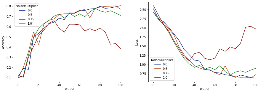
ปรากฏว่ามีลูกค้าคาดหวัง 50 รายต่อรอบ โมเดลนี้สามารถทนต่อตัวคูณเสียงรบกวนได้สูงถึง 0.5 โดยไม่ลดคุณภาพของโมเดล ตัวคูณสัญญาณรบกวน 0.75 ดูเหมือนจะทำให้โมเดลเสื่อมโทรมเล็กน้อย และ 1.0 ทำให้โมเดลแตกต่างออกไป
โดยทั่วไปจะมีการแลกเปลี่ยนระหว่างคุณภาพของแบบจำลองและความเป็นส่วนตัว ยิ่งเราใช้เสียงรบกวนมากเท่าไร เราก็ยิ่งได้รับความเป็นส่วนตัวมากขึ้นเท่านั้นสำหรับเวลาการฝึกอบรมและจำนวนลูกค้าที่เท่ากัน ในทางกลับกัน หากเสียงรบกวนน้อยลง เราอาจมีโมเดลที่แม่นยำกว่า แต่เราจะต้องฝึกอบรมกับลูกค้ามากขึ้นในแต่ละรอบเพื่อให้ถึงระดับความเป็นส่วนตัวเป้าหมายของเรา
จากการทดลองข้างต้น เราอาจตัดสินใจว่าการเสื่อมสภาพของแบบจำลองจำนวนเล็กน้อยที่ 0.75 นั้นเป็นที่ยอมรับได้ เพื่อที่จะฝึกโมเดลสุดท้ายให้เร็วขึ้น แต่สมมติว่าเราต้องการจับคู่ประสิทธิภาพของโมเดลตัวคูณสัญญาณรบกวน 0.5
ตอนนี้ เราสามารถใช้ฟังก์ชัน tensorflow_privacy เพื่อกำหนดจำนวนลูกค้าที่คาดหวังต่อรอบ เราจะต้องได้รับความเป็นส่วนตัวที่ยอมรับได้ แนวปฏิบัติมาตรฐานคือการเลือกเดลต้าที่ค่อนข้างเล็กกว่าหนึ่งในจำนวนเร็กคอร์ดในชุดข้อมูล ชุดข้อมูลนี้มีผู้ใช้การฝึกทั้งหมด 3383 คน ดังนั้นเรามาตั้งเป้า (2, 1e-5)-DP กัน
เราใช้การค้นหาแบบไบนารีอย่างง่ายกับจำนวนลูกค้าต่อรอบ ฟังก์ชั่น tensorflow_privacy เราใช้ในการประเมิน epsilon จะขึ้นอยู่กับ วัง et al, (2018) และ Mironov et al, (2019)
rdp_orders = ([1.25, 1.5, 1.75, 2., 2.25, 2.5, 3., 3.5, 4., 4.5] +
              list(range(5, 64)) + [128, 256, 512])

total_clients = 3383
base_noise_multiplier = 0.5
base_clients_per_round = 50
target_delta = 1e-5
target_eps = 2

def get_epsilon(clients_per_round):
  # If we use this number of clients per round and proportionally
  # scale up the noise multiplier, what epsilon do we achieve?
  q = clients_per_round / total_clients
  noise_multiplier = base_noise_multiplier
  noise_multiplier *= clients_per_round / base_clients_per_round
  rdp = tfp.compute_rdp(
      q, noise_multiplier=noise_multiplier, steps=rounds, orders=rdp_orders)
  eps, _, _ = tfp.get_privacy_spent(rdp_orders, rdp, target_delta=target_delta)
  return clients_per_round, eps, noise_multiplier

def find_needed_clients_per_round():
  hi = get_epsilon(base_clients_per_round)
  if hi[1] < target_eps:
    return hi

  # Grow interval exponentially until target_eps is exceeded.
  while True:
    lo = hi
    hi = get_epsilon(2 * lo[0])
    if hi[1] < target_eps:
      break

  # Binary search.
  while hi[0] - lo[0] > 1:
    mid = get_epsilon((lo[0] + hi[0]) // 2)
    if mid[1] > target_eps:
      lo = mid
    else:
      hi = mid

  return hi

clients_per_round, _, noise_multiplier = find_needed_clients_per_round()
print(f'To get ({target_eps}, {target_delta})-DP, use {clients_per_round} '
      f'clients with noise multiplier {noise_multiplier}.')
To get (2, 1e-05)-DP, use 120 clients with noise multiplier 1.2.
ตอนนี้ เราสามารถฝึกโมเดลส่วนตัวขั้นสุดท้ายสำหรับการเปิดตัวได้
rounds = 100
noise_multiplier = 1.2
clients_per_round = 120

data_frame = pd.DataFrame()
data_frame = train(rounds, noise_multiplier, clients_per_round, data_frame)

make_plot(data_frame)
Round   0: OrderedDict([('sparse_categorical_accuracy', 0.08260678), ('loss', 2.6334999)])
Round   5: OrderedDict([('sparse_categorical_accuracy', 0.1492212), ('loss', 2.259542)])
Round  10: OrderedDict([('sparse_categorical_accuracy', 0.28847474), ('loss', 2.155699)])
Round  15: OrderedDict([('sparse_categorical_accuracy', 0.3989518), ('loss', 2.0156953)])
Round  20: OrderedDict([('sparse_categorical_accuracy', 0.5086697), ('loss', 1.8261365)])
Round  25: OrderedDict([('sparse_categorical_accuracy', 0.6204692), ('loss', 1.5602393)])
Round  50: OrderedDict([('sparse_categorical_accuracy', 0.70008814), ('loss', 0.91155165)])
Round  75: OrderedDict([('sparse_categorical_accuracy', 0.78421336), ('loss', 0.6820159)])
Round 100: OrderedDict([('sparse_categorical_accuracy', 0.7955525), ('loss', 0.6585961)])
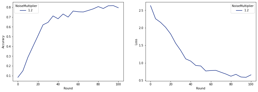
ดังที่เราเห็น โมเดลสุดท้ายมีความสูญเสียและความแม่นยำคล้ายกับรุ่นที่ฝึกโดยไม่มีเสียงรบกวน แต่รุ่นนี้ตอบสนอง (2, 1e-5)-DP