Advanced automatic differentiation

The Introduction to gradients and automatic differentiation guide includes everything required to calculate gradients in TensorFlow. This guide focuses on deeper, less common features of the tf.GradientTape API.

Setup

import tensorflow as tf

import matplotlib as mpl
import matplotlib.pyplot as plt

mpl.rcParams['figure.figsize'] = (8, 6)

2024-07-19 02:50:43.916438: E external/local_xla/xla/stream_executor/cuda/cuda_fft.cc:485] Unable to register cuFFT factory: Attempting to register factory for plugin cuFFT when one has already been registered
2024-07-19 02:50:43.937690: E external/local_xla/xla/stream_executor/cuda/cuda_dnn.cc:8454] Unable to register cuDNN factory: Attempting to register factory for plugin cuDNN when one has already been registered
2024-07-19 02:50:43.944003: E external/local_xla/xla/stream_executor/cuda/cuda_blas.cc:1452] Unable to register cuBLAS factory: Attempting to register factory for plugin cuBLAS when one has already been registered

Controlling gradient recording

In the automatic differentiation guide you saw how to control which variables and tensors are watched by the tape while building the gradient calculation.

The tape also has methods to manipulate the recording.

Stop recording

If you wish to stop recording gradients, you can use tf.GradientTape.stop_recording to temporarily suspend recording.

This may be useful to reduce overhead if you do not wish to differentiate a complicated operation in the middle of your model. This could include calculating a metric or an intermediate result:

x = tf.Variable(2.0)
y = tf.Variable(3.0)

with tf.GradientTape() as t:
  x_sq = x * x
  with t.stop_recording():
    y_sq = y * y
  z = x_sq + y_sq

grad = t.gradient(z, {'x': x, 'y': y})

print('dz/dx:', grad['x'])  # 2*x => 4
print('dz/dy:', grad['y'])

dz/dx: tf.Tensor(4.0, shape=(), dtype=float32)
dz/dy: None
WARNING: All log messages before absl::InitializeLog() is called are written to STDERR
I0000 00:00:1721357446.860587  136363 cuda_executor.cc:1015] successful NUMA node read from SysFS had negative value (-1), but there must be at least one NUMA node, so returning NUMA node zero. See more at https://github.com/torvalds/linux/blob/v6.0/Documentation/ABI/testing/sysfs-bus-pci#L344-L355
I0000 00:00:1721357446.864384  136363 cuda_executor.cc:1015] successful NUMA node read from SysFS had negative value (-1), but there must be at least one NUMA node, so returning NUMA node zero. See more at https://github.com/torvalds/linux/blob/v6.0/Documentation/ABI/testing/sysfs-bus-pci#L344-L355
I0000 00:00:1721357446.868144  136363 cuda_executor.cc:1015] successful NUMA node read from SysFS had negative value (-1), but there must be at least one NUMA node, so returning NUMA node zero. See more at https://github.com/torvalds/linux/blob/v6.0/Documentation/ABI/testing/sysfs-bus-pci#L344-L355
I0000 00:00:1721357446.871707  136363 cuda_executor.cc:1015] successful NUMA node read from SysFS had negative value (-1), but there must be at least one NUMA node, so returning NUMA node zero. See more at https://github.com/torvalds/linux/blob/v6.0/Documentation/ABI/testing/sysfs-bus-pci#L344-L355
I0000 00:00:1721357446.884190  136363 cuda_executor.cc:1015] successful NUMA node read from SysFS had negative value (-1), but there must be at least one NUMA node, so returning NUMA node zero. See more at https://github.com/torvalds/linux/blob/v6.0/Documentation/ABI/testing/sysfs-bus-pci#L344-L355
I0000 00:00:1721357446.887603  136363 cuda_executor.cc:1015] successful NUMA node read from SysFS had negative value (-1), but there must be at least one NUMA node, so returning NUMA node zero. See more at https://github.com/torvalds/linux/blob/v6.0/Documentation/ABI/testing/sysfs-bus-pci#L344-L355
I0000 00:00:1721357446.891098  136363 cuda_executor.cc:1015] successful NUMA node read from SysFS had negative value (-1), but there must be at least one NUMA node, so returning NUMA node zero. See more at https://github.com/torvalds/linux/blob/v6.0/Documentation/ABI/testing/sysfs-bus-pci#L344-L355
I0000 00:00:1721357446.894451  136363 cuda_executor.cc:1015] successful NUMA node read from SysFS had negative value (-1), but there must be at least one NUMA node, so returning NUMA node zero. See more at https://github.com/torvalds/linux/blob/v6.0/Documentation/ABI/testing/sysfs-bus-pci#L344-L355
I0000 00:00:1721357446.897962  136363 cuda_executor.cc:1015] successful NUMA node read from SysFS had negative value (-1), but there must be at least one NUMA node, so returning NUMA node zero. See more at https://github.com/torvalds/linux/blob/v6.0/Documentation/ABI/testing/sysfs-bus-pci#L344-L355
I0000 00:00:1721357446.901403  136363 cuda_executor.cc:1015] successful NUMA node read from SysFS had negative value (-1), but there must be at least one NUMA node, so returning NUMA node zero. See more at https://github.com/torvalds/linux/blob/v6.0/Documentation/ABI/testing/sysfs-bus-pci#L344-L355
I0000 00:00:1721357446.904883  136363 cuda_executor.cc:1015] successful NUMA node read from SysFS had negative value (-1), but there must be at least one NUMA node, so returning NUMA node zero. See more at https://github.com/torvalds/linux/blob/v6.0/Documentation/ABI/testing/sysfs-bus-pci#L344-L355
I0000 00:00:1721357446.908301  136363 cuda_executor.cc:1015] successful NUMA node read from SysFS had negative value (-1), but there must be at least one NUMA node, so returning NUMA node zero. See more at https://github.com/torvalds/linux/blob/v6.0/Documentation/ABI/testing/sysfs-bus-pci#L344-L355
I0000 00:00:1721357448.171935  136363 cuda_executor.cc:1015] successful NUMA node read from SysFS had negative value (-1), but there must be at least one NUMA node, so returning NUMA node zero. See more at https://github.com/torvalds/linux/blob/v6.0/Documentation/ABI/testing/sysfs-bus-pci#L344-L355
I0000 00:00:1721357448.174025  136363 cuda_executor.cc:1015] successful NUMA node read from SysFS had negative value (-1), but there must be at least one NUMA node, so returning NUMA node zero. See more at https://github.com/torvalds/linux/blob/v6.0/Documentation/ABI/testing/sysfs-bus-pci#L344-L355
I0000 00:00:1721357448.175971  136363 cuda_executor.cc:1015] successful NUMA node read from SysFS had negative value (-1), but there must be at least one NUMA node, so returning NUMA node zero. See more at https://github.com/torvalds/linux/blob/v6.0/Documentation/ABI/testing/sysfs-bus-pci#L344-L355
I0000 00:00:1721357448.177986  136363 cuda_executor.cc:1015] successful NUMA node read from SysFS had negative value (-1), but there must be at least one NUMA node, so returning NUMA node zero. See more at https://github.com/torvalds/linux/blob/v6.0/Documentation/ABI/testing/sysfs-bus-pci#L344-L355
I0000 00:00:1721357448.180036  136363 cuda_executor.cc:1015] successful NUMA node read from SysFS had negative value (-1), but there must be at least one NUMA node, so returning NUMA node zero. See more at https://github.com/torvalds/linux/blob/v6.0/Documentation/ABI/testing/sysfs-bus-pci#L344-L355
I0000 00:00:1721357448.181937  136363 cuda_executor.cc:1015] successful NUMA node read from SysFS had negative value (-1), but there must be at least one NUMA node, so returning NUMA node zero. See more at https://github.com/torvalds/linux/blob/v6.0/Documentation/ABI/testing/sysfs-bus-pci#L344-L355
I0000 00:00:1721357448.183763  136363 cuda_executor.cc:1015] successful NUMA node read from SysFS had negative value (-1), but there must be at least one NUMA node, so returning NUMA node zero. See more at https://github.com/torvalds/linux/blob/v6.0/Documentation/ABI/testing/sysfs-bus-pci#L344-L355
I0000 00:00:1721357448.185685  136363 cuda_executor.cc:1015] successful NUMA node read from SysFS had negative value (-1), but there must be at least one NUMA node, so returning NUMA node zero. See more at https://github.com/torvalds/linux/blob/v6.0/Documentation/ABI/testing/sysfs-bus-pci#L344-L355
I0000 00:00:1721357448.187626  136363 cuda_executor.cc:1015] successful NUMA node read from SysFS had negative value (-1), but there must be at least one NUMA node, so returning NUMA node zero. See more at https://github.com/torvalds/linux/blob/v6.0/Documentation/ABI/testing/sysfs-bus-pci#L344-L355
I0000 00:00:1721357448.189545  136363 cuda_executor.cc:1015] successful NUMA node read from SysFS had negative value (-1), but there must be at least one NUMA node, so returning NUMA node zero. See more at https://github.com/torvalds/linux/blob/v6.0/Documentation/ABI/testing/sysfs-bus-pci#L344-L355
I0000 00:00:1721357448.191377  136363 cuda_executor.cc:1015] successful NUMA node read from SysFS had negative value (-1), but there must be at least one NUMA node, so returning NUMA node zero. See more at https://github.com/torvalds/linux/blob/v6.0/Documentation/ABI/testing/sysfs-bus-pci#L344-L355
I0000 00:00:1721357448.193295  136363 cuda_executor.cc:1015] successful NUMA node read from SysFS had negative value (-1), but there must be at least one NUMA node, so returning NUMA node zero. See more at https://github.com/torvalds/linux/blob/v6.0/Documentation/ABI/testing/sysfs-bus-pci#L344-L355
I0000 00:00:1721357448.231363  136363 cuda_executor.cc:1015] successful NUMA node read from SysFS had negative value (-1), but there must be at least one NUMA node, so returning NUMA node zero. See more at https://github.com/torvalds/linux/blob/v6.0/Documentation/ABI/testing/sysfs-bus-pci#L344-L355
I0000 00:00:1721357448.233482  136363 cuda_executor.cc:1015] successful NUMA node read from SysFS had negative value (-1), but there must be at least one NUMA node, so returning NUMA node zero. See more at https://github.com/torvalds/linux/blob/v6.0/Documentation/ABI/testing/sysfs-bus-pci#L344-L355
I0000 00:00:1721357448.235953  136363 cuda_executor.cc:1015] successful NUMA node read from SysFS had negative value (-1), but there must be at least one NUMA node, so returning NUMA node zero. See more at https://github.com/torvalds/linux/blob/v6.0/Documentation/ABI/testing/sysfs-bus-pci#L344-L355
I0000 00:00:1721357448.237931  136363 cuda_executor.cc:1015] successful NUMA node read from SysFS had negative value (-1), but there must be at least one NUMA node, so returning NUMA node zero. See more at https://github.com/torvalds/linux/blob/v6.0/Documentation/ABI/testing/sysfs-bus-pci#L344-L355
I0000 00:00:1721357448.239900  136363 cuda_executor.cc:1015] successful NUMA node read from SysFS had negative value (-1), but there must be at least one NUMA node, so returning NUMA node zero. See more at https://github.com/torvalds/linux/blob/v6.0/Documentation/ABI/testing/sysfs-bus-pci#L344-L355
I0000 00:00:1721357448.241810  136363 cuda_executor.cc:1015] successful NUMA node read from SysFS had negative value (-1), but there must be at least one NUMA node, so returning NUMA node zero. See more at https://github.com/torvalds/linux/blob/v6.0/Documentation/ABI/testing/sysfs-bus-pci#L344-L355
I0000 00:00:1721357448.243663  136363 cuda_executor.cc:1015] successful NUMA node read from SysFS had negative value (-1), but there must be at least one NUMA node, so returning NUMA node zero. See more at https://github.com/torvalds/linux/blob/v6.0/Documentation/ABI/testing/sysfs-bus-pci#L344-L355
I0000 00:00:1721357448.245603  136363 cuda_executor.cc:1015] successful NUMA node read from SysFS had negative value (-1), but there must be at least one NUMA node, so returning NUMA node zero. See more at https://github.com/torvalds/linux/blob/v6.0/Documentation/ABI/testing/sysfs-bus-pci#L344-L355
I0000 00:00:1721357448.247582  136363 cuda_executor.cc:1015] successful NUMA node read from SysFS had negative value (-1), but there must be at least one NUMA node, so returning NUMA node zero. See more at https://github.com/torvalds/linux/blob/v6.0/Documentation/ABI/testing/sysfs-bus-pci#L344-L355
I0000 00:00:1721357448.249942  136363 cuda_executor.cc:1015] successful NUMA node read from SysFS had negative value (-1), but there must be at least one NUMA node, so returning NUMA node zero. See more at https://github.com/torvalds/linux/blob/v6.0/Documentation/ABI/testing/sysfs-bus-pci#L344-L355
I0000 00:00:1721357448.252134  136363 cuda_executor.cc:1015] successful NUMA node read from SysFS had negative value (-1), but there must be at least one NUMA node, so returning NUMA node zero. See more at https://github.com/torvalds/linux/blob/v6.0/Documentation/ABI/testing/sysfs-bus-pci#L344-L355
I0000 00:00:1721357448.254535  136363 cuda_executor.cc:1015] successful NUMA node read from SysFS had negative value (-1), but there must be at least one NUMA node, so returning NUMA node zero. See more at https://github.com/torvalds/linux/blob/v6.0/Documentation/ABI/testing/sysfs-bus-pci#L344-L355

Reset/start recording from scratch

If you wish to start over entirely, use tf.GradientTape.reset. Simply exiting the gradient tape block and restarting is usually easier to read, but you can use the reset method when exiting the tape block is difficult or impossible.

x = tf.Variable(2.0)
y = tf.Variable(3.0)
reset = True

with tf.GradientTape() as t:
  y_sq = y * y
  if reset:
    # Throw out all the tape recorded so far.
    t.reset()
  z = x * x + y_sq

grad = t.gradient(z, {'x': x, 'y': y})

print('dz/dx:', grad['x'])  # 2*x => 4
print('dz/dy:', grad['y'])

dz/dx: tf.Tensor(4.0, shape=(), dtype=float32)
dz/dy: None

Stop gradient flow with precision

In contrast to the global tape controls above, the tf.stop_gradient function is much more precise. It can be used to stop gradients from flowing along a particular path, without needing access to the tape itself:

x = tf.Variable(2.0)
y = tf.Variable(3.0)

with tf.GradientTape() as t:
  y_sq = y**2
  z = x**2 + tf.stop_gradient(y_sq)

grad = t.gradient(z, {'x': x, 'y': y})

print('dz/dx:', grad['x'])  # 2*x => 4
print('dz/dy:', grad['y'])

dz/dx: tf.Tensor(4.0, shape=(), dtype=float32)
dz/dy: None

Custom gradients

In some cases, you may want to control exactly how gradients are calculated rather than using the default. These situations include:

1. There is no defined gradient for a new op you are writing.
2. The default calculations are numerically unstable.
3. You wish to cache an expensive computation from the forward pass.
4. You want to modify a value (for example, using tf.clip_by_value or tf.math.round) without modifying the gradient.

For the first case, to write a new op you can use tf.RegisterGradient to set up your own (refer to the API docs for details). (Note that the gradient registry is global, so change it with caution.)

For the latter three cases, you can use tf.custom_gradient.

Here is an example that applies tf.clip_by_norm to the intermediate gradient:

# Establish an identity operation, but clip during the gradient pass.
@tf.custom_gradient
def clip_gradients(y):
  def backward(dy):
    return tf.clip_by_norm(dy, 0.5)
  return y, backward

v = tf.Variable(2.0)
with tf.GradientTape() as t:
  output = clip_gradients(v * v)
print(t.gradient(output, v))  # calls "backward", which clips 4 to 2

tf.Tensor(2.0, shape=(), dtype=float32)

Refer to the tf.custom_gradient decorator API docs for more details.

Custom gradients in SavedModel

Note: This feature is available from TensorFlow 2.6.

Custom gradients can be saved to SavedModel by using the option tf.saved_model.SaveOptions(experimental_custom_gradients=True).

To be saved into the SavedModel, the gradient function must be traceable (to learn more, check out the Better performance with tf.function guide).

class MyModule(tf.Module):

  @tf.function(input_signature=[tf.TensorSpec(None)])
  def call_custom_grad(self, x):
    return clip_gradients(x)

model = MyModule()

tf.saved_model.save(
    model,
    'saved_model',
    options=tf.saved_model.SaveOptions(experimental_custom_gradients=True))

# The loaded gradients will be the same as the above example.
v = tf.Variable(2.0)
loaded = tf.saved_model.load('saved_model')
with tf.GradientTape() as t:
  output = loaded.call_custom_grad(v * v)
print(t.gradient(output, v))

INFO:tensorflow:Assets written to: saved_model/assets
INFO:tensorflow:Assets written to: saved_model/assets
tf.Tensor(2.0, shape=(), dtype=float32)

A note about the above example: If you try replacing the above code with tf.saved_model.SaveOptions(experimental_custom_gradients=False), the gradient will still produce the same result on loading. The reason is that the gradient registry still contains the custom gradient used in the function call_custom_op. However, if you restart the runtime after saving without custom gradients, running the loaded model under the tf.GradientTape will throw the error: LookupError: No gradient defined for operation 'IdentityN' (op type: IdentityN).

Multiple tapes

Multiple tapes interact seamlessly.

For example, here each tape watches a different set of tensors:

x0 = tf.constant(0.0)
x1 = tf.constant(0.0)

with tf.GradientTape() as tape0, tf.GradientTape() as tape1:
  tape0.watch(x0)
  tape1.watch(x1)

  y0 = tf.math.sin(x0)
  y1 = tf.nn.sigmoid(x1)

  y = y0 + y1

  ys = tf.reduce_sum(y)

tape0.gradient(ys, x0).numpy()   # cos(x) => 1.0

1.0

tape1.gradient(ys, x1).numpy()   # sigmoid(x1)*(1-sigmoid(x1)) => 0.25

0.25

Higher-order gradients

Operations inside of the tf.GradientTape context manager are recorded for automatic differentiation. If gradients are computed in that context, then the gradient computation is recorded as well. As a result, the exact same API works for higher-order gradients as well.

For example:

x = tf.Variable(1.0)  # Create a Tensorflow variable initialized to 1.0

with tf.GradientTape() as t2:
  with tf.GradientTape() as t1:
    y = x * x * x

  # Compute the gradient inside the outer `t2` context manager
  # which means the gradient computation is differentiable as well.
  dy_dx = t1.gradient(y, x)
d2y_dx2 = t2.gradient(dy_dx, x)

print('dy_dx:', dy_dx.numpy())  # 3 * x**2 => 3.0
print('d2y_dx2:', d2y_dx2.numpy())  # 6 * x => 6.0

dy_dx: 3.0
d2y_dx2: 6.0

While that does give you the second derivative of a scalar function, this pattern does not generalize to produce a Hessian matrix, since tf.GradientTape.gradient only computes the gradient of a scalar. To construct a Hessian matrix, go to the Hessian example under the Jacobian section.

"Nested calls to tf.GradientTape.gradient" is a good pattern when you are calculating a scalar from a gradient, and then the resulting scalar acts as a source for a second gradient calculation, as in the following example.

Example: Input gradient regularization

Many models are susceptible to "adversarial examples". This collection of techniques modifies the model's input to confuse the model's output. The simplest implementation—such as the Adversarial example using the Fast Gradient Signed Method attack—takes a single step along the gradient of the output with respect to the input; the "input gradient".

One technique to increase robustness to adversarial examples is input gradient regularization (Finlay & Oberman, 2019), which attempts to minimize the magnitude of the input gradient. If the input gradient is small, then the change in the output should be small too.

Below is a naive implementation of input gradient regularization. The implementation is:

1. Calculate the gradient of the output with respect to the input using an inner tape.
2. Calculate the magnitude of that input gradient.
3. Calculate the gradient of that magnitude with respect to the model.

x = tf.random.normal([7, 5])

layer = tf.keras.layers.Dense(10, activation=tf.nn.relu)

with tf.GradientTape() as t2:
  # The inner tape only takes the gradient with respect to the input,
  # not the variables.
  with tf.GradientTape(watch_accessed_variables=False) as t1:
    t1.watch(x)
    y = layer(x)
    out = tf.reduce_sum(layer(x)**2)
  # 1. Calculate the input gradient.
  g1 = t1.gradient(out, x)
  # 2. Calculate the magnitude of the input gradient.
  g1_mag = tf.norm(g1)

# 3. Calculate the gradient of the magnitude with respect to the model.
dg1_mag = t2.gradient(g1_mag, layer.trainable_variables)

[var.shape for var in dg1_mag]

[TensorShape([5, 10]), TensorShape([10])]

Jacobians

All the previous examples took the gradients of a scalar target with respect to some source tensor(s).

The Jacobian matrix represents the gradients of a vector valued function. Each row contains the gradient of one of the vector's elements.

The tf.GradientTape.jacobian method allows you to efficiently calculate a Jacobian matrix.

Note that:

• Like gradient: The sources argument can be a tensor or a container of tensors.
• Unlike gradient: The target tensor must be a single tensor.

Scalar source

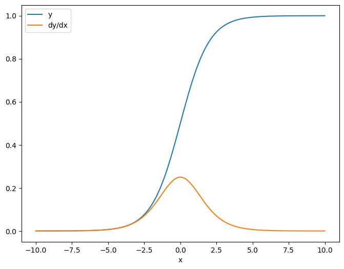
As a first example, here is the Jacobian of a vector-target with respect to a scalar-source.

x = tf.linspace(-10.0, 10.0, 200+1)
delta = tf.Variable(0.0)

with tf.GradientTape() as tape:
  y = tf.nn.sigmoid(x+delta)

dy_dx = tape.jacobian(y, delta)

When you take the Jacobian with respect to a scalar the result has the shape of the target, and gives the gradient of the each element with respect to the source:

print(y.shape)
print(dy_dx.shape)

(201,)
(201,)

plt.plot(x.numpy(), y, label='y')
plt.plot(x.numpy(), dy_dx, label='dy/dx')
plt.legend()
_ = plt.xlabel('x')

Tensor source

Whether the input is scalar or tensor, tf.GradientTape.jacobian efficiently calculates the gradient of each element of the source with respect to each element of the target(s).

For example, the output of this layer has a shape of (10, 7):

x = tf.random.normal([7, 5])
layer = tf.keras.layers.Dense(10, activation=tf.nn.relu)

with tf.GradientTape(persistent=True) as tape:
  y = layer(x)

y.shape

TensorShape([7, 10])

And the layer's kernel's shape is (5, 10):

layer.kernel.shape

TensorShape([5, 10])

The shape of the Jacobian of the output with respect to the kernel is those two shapes concatenated together:

j = tape.jacobian(y, layer.kernel)
j.shape

TensorShape([7, 10, 5, 10])

If you sum over the target's dimensions, you're left with the gradient of the sum that would have been calculated by tf.GradientTape.gradient:

g = tape.gradient(y, layer.kernel)
print('g.shape:', g.shape)

j_sum = tf.reduce_sum(j, axis=[0, 1])
delta = tf.reduce_max(abs(g - j_sum)).numpy()
assert delta < 1e-3
print('delta:', delta)

g.shape: (5, 10)
delta: 2.3841858e-07

Example: Hessian

While tf.GradientTape doesn't give an explicit method for constructing a Hessian matrix it's possible to build one using the tf.GradientTape.jacobian method.

Note: The Hessian matrix contains N**2 parameters. For this and other reasons it is not practical for most models. This example is included more as a demonstration of how to use the tf.GradientTape.jacobian method, and is not an endorsement of direct Hessian-based optimization. A Hessian-vector product can be calculated efficiently with nested tapes, and is a much more efficient approach to second-order optimization.

x = tf.random.normal([7, 5])
layer1 = tf.keras.layers.Dense(8, activation=tf.nn.relu)
layer2 = tf.keras.layers.Dense(6, activation=tf.nn.relu)

with tf.GradientTape() as t2:
  with tf.GradientTape() as t1:
    x = layer1(x)
    x = layer2(x)
    loss = tf.reduce_mean(x**2)

  g = t1.gradient(loss, layer1.kernel)

h = t2.jacobian(g, layer1.kernel)

print(f'layer.kernel.shape: {layer1.kernel.shape}')
print(f'h.shape: {h.shape}')

layer.kernel.shape: (5, 8)
h.shape: (5, 8, 5, 8)

To use this Hessian for a Newton's method step, you would first flatten out its axes into a matrix, and flatten out the gradient into a vector:

n_params = tf.reduce_prod(layer1.kernel.shape)

g_vec = tf.reshape(g, [n_params, 1])
h_mat = tf.reshape(h, [n_params, n_params])

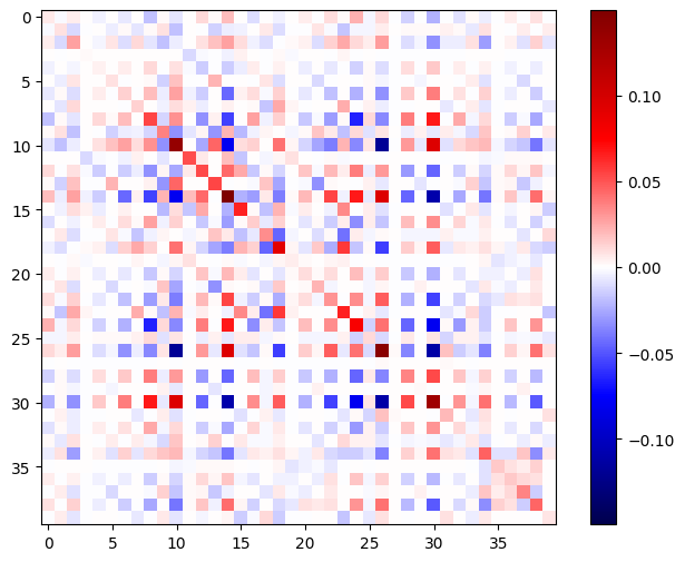
The Hessian matrix should be symmetric:

def imshow_zero_center(image, **kwargs):
  lim = tf.reduce_max(abs(image))
  plt.imshow(image, vmin=-lim, vmax=lim, cmap='seismic', **kwargs)
  plt.colorbar()

imshow_zero_center(h_mat)

The Newton's method update step is shown below:

eps = 1e-3
eye_eps = tf.eye(h_mat.shape[0])*eps

Note: Don't actually invert the matrix.

# X(k+1) = X(k) - (∇²f(X(k)))^-1 @ ∇f(X(k))
# h_mat = ∇²f(X(k))
# g_vec = ∇f(X(k))
update = tf.linalg.solve(h_mat + eye_eps, g_vec)

# Reshape the update and apply it to the variable.
_ = layer1.kernel.assign_sub(tf.reshape(update, layer1.kernel.shape))

While this is relatively simple for a single tf.Variable, applying this to a non-trivial model would require careful concatenation and slicing to produce a full Hessian across multiple variables.

Batch Jacobian

In some cases, you want to take the Jacobian of each of a stack of targets with respect to a stack of sources, where the Jacobians for each target-source pair are independent.

For example, here the input x is shaped (batch, ins) and the output y is shaped (batch, outs):

x = tf.random.normal([7, 5])

layer1 = tf.keras.layers.Dense(8, activation=tf.nn.elu)
layer2 = tf.keras.layers.Dense(6, activation=tf.nn.elu)

with tf.GradientTape(persistent=True, watch_accessed_variables=False) as tape:
  tape.watch(x)
  y = layer1(x)
  y = layer2(y)

y.shape

TensorShape([7, 6])

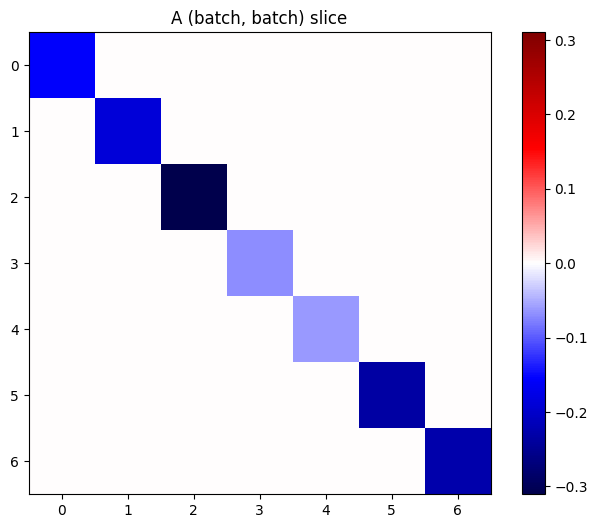
The full Jacobian of y with respect to x has a shape of (batch, ins, batch, outs), even if you only want (batch, ins, outs):

j = tape.jacobian(y, x)
j.shape

TensorShape([7, 6, 7, 5])

If the gradients of each item in the stack are independent, then every (batch, batch) slice of this tensor is a diagonal matrix:

imshow_zero_center(j[:, 0, :, 0])
_ = plt.title('A (batch, batch) slice')

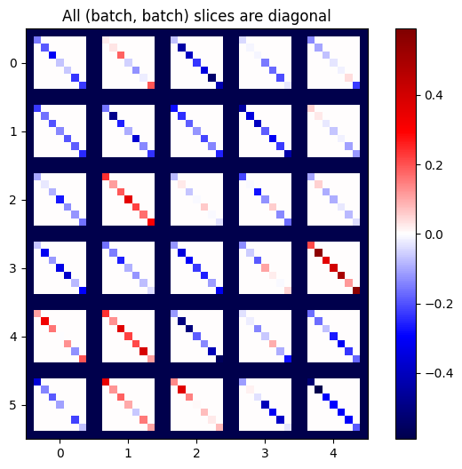
def plot_as_patches(j):
  # Reorder axes so the diagonals will each form a contiguous patch.
  j = tf.transpose(j, [1, 0, 3, 2])
  # Pad in between each patch.
  lim = tf.reduce_max(abs(j))
  j = tf.pad(j, [[0, 0], [1, 1], [0, 0], [1, 1]],
             constant_values=-lim)
  # Reshape to form a single image.
  s = j.shape
  j = tf.reshape(j, [s[0]*s[1], s[2]*s[3]])
  imshow_zero_center(j, extent=[-0.5, s[2]-0.5, s[0]-0.5, -0.5])

plot_as_patches(j)
_ = plt.title('All (batch, batch) slices are diagonal')

To get the desired result, you can sum over the duplicate batch dimension, or else select the diagonals using tf.einsum:

j_sum = tf.reduce_sum(j, axis=2)
print(j_sum.shape)
j_select = tf.einsum('bxby->bxy', j)
print(j_select.shape)

(7, 6, 5)
(7, 6, 5)

It would be much more efficient to do the calculation without the extra dimension in the first place. The tf.GradientTape.batch_jacobian method does exactly that:

jb = tape.batch_jacobian(y, x)
jb.shape

WARNING:tensorflow:5 out of the last 5 calls to <function pfor.<locals>.f at 0x7fb3886ecca0> triggered tf.function retracing. Tracing is expensive and the excessive number of tracings could be due to (1) creating @tf.function repeatedly in a loop, (2) passing tensors with different shapes, (3) passing Python objects instead of tensors. For (1), please define your @tf.function outside of the loop. For (2), @tf.function has reduce_retracing=True option that can avoid unnecessary retracing. For (3), please refer to https://www.tensorflow.org/guide/function#controlling_retracing and https://www.tensorflow.org/api_docs/python/tf/function for  more details.
WARNING:tensorflow:5 out of the last 5 calls to <function pfor.<locals>.f at 0x7fb3886ecca0> triggered tf.function retracing. Tracing is expensive and the excessive number of tracings could be due to (1) creating @tf.function repeatedly in a loop, (2) passing tensors with different shapes, (3) passing Python objects instead of tensors. For (1), please define your @tf.function outside of the loop. For (2), @tf.function has reduce_retracing=True option that can avoid unnecessary retracing. For (3), please refer to https://www.tensorflow.org/guide/function#controlling_retracing and https://www.tensorflow.org/api_docs/python/tf/function for  more details.
TensorShape([7, 6, 5])

error = tf.reduce_max(abs(jb - j_sum))
assert error < 1e-3
print(error.numpy())

0.0

Caution: tf.GradientTape.batch_jacobian only verifies that the first dimension of the source and target match. It doesn't check that the gradients are actually independent. It's up to you to make sure you only use batch_jacobian where it makes sense. For example, adding a tf.keras.layers.BatchNormalization destroys the independence, since it normalizes across the batch dimension:

x = tf.random.normal([7, 5])

layer1 = tf.keras.layers.Dense(8, activation=tf.nn.elu)
bn = tf.keras.layers.BatchNormalization()
layer2 = tf.keras.layers.Dense(6, activation=tf.nn.elu)

with tf.GradientTape(persistent=True, watch_accessed_variables=False) as tape:
  tape.watch(x)
  y = layer1(x)
  y = bn(y, training=True)
  y = layer2(y)

j = tape.jacobian(y, x)
print(f'j.shape: {j.shape}')

WARNING:tensorflow:6 out of the last 6 calls to <function pfor.<locals>.f at 0x7fb3886ec9d0> triggered tf.function retracing. Tracing is expensive and the excessive number of tracings could be due to (1) creating @tf.function repeatedly in a loop, (2) passing tensors with different shapes, (3) passing Python objects instead of tensors. For (1), please define your @tf.function outside of the loop. For (2), @tf.function has reduce_retracing=True option that can avoid unnecessary retracing. For (3), please refer to https://www.tensorflow.org/guide/function#controlling_retracing and https://www.tensorflow.org/api_docs/python/tf/function for  more details.
WARNING:tensorflow:6 out of the last 6 calls to <function pfor.<locals>.f at 0x7fb3886ec9d0> triggered tf.function retracing. Tracing is expensive and the excessive number of tracings could be due to (1) creating @tf.function repeatedly in a loop, (2) passing tensors with different shapes, (3) passing Python objects instead of tensors. For (1), please define your @tf.function outside of the loop. For (2), @tf.function has reduce_retracing=True option that can avoid unnecessary retracing. For (3), please refer to https://www.tensorflow.org/guide/function#controlling_retracing and https://www.tensorflow.org/api_docs/python/tf/function for  more details.
j.shape: (7, 6, 7, 5)

plot_as_patches(j)

_ = plt.title('These slices are not diagonal')
_ = plt.xlabel("Don't use `batch_jacobian`")

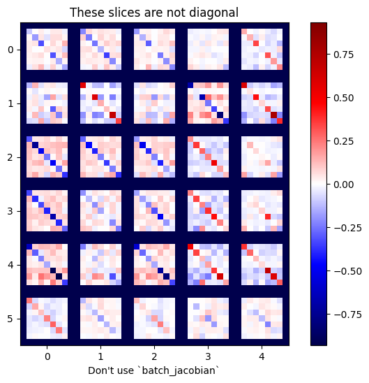
In this case, batch_jacobian still runs and returns something with the expected shape, but its contents have an unclear meaning:

jb = tape.batch_jacobian(y, x)
print(f'jb.shape: {jb.shape}')

jb.shape: (7, 6, 5)