|
|
|
 View source on GitHub View source on GitHub
|
|
This notebook demonstrates the use of TFP approximate inference tools to incorporate a (non-Gaussian) observation model when fitting and forecasting with structural time series (STS) models. In this example, we'll use a Poisson observation model to work with discrete count data.
import time
import matplotlib.pyplot as plt
import numpy as np

import tensorflow as tf
import tf_keras
import tensorflow_probability as tfp

from tensorflow_probability import bijectors as tfb
from tensorflow_probability import distributions as tfd
Synthetic Data
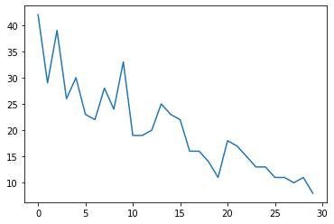
First we'll generate some synthetic count data:
num_timesteps = 30
observed_counts = np.round(3 + np.random.lognormal(np.log(np.linspace(
    num_timesteps, 5, num=num_timesteps)), 0.20, size=num_timesteps))
observed_counts = observed_counts.astype(np.float32)
plt.plot(observed_counts)
[<matplotlib.lines.Line2D at 0x7f940ae958d0>]
Model
We'll specify a simple model with a randomly walking linear trend:
def build_model(approximate_unconstrained_rates):
  trend = tfp.sts.LocalLinearTrend(
      observed_time_series=approximate_unconstrained_rates)
  return tfp.sts.Sum([trend],
                     observed_time_series=approximate_unconstrained_rates)
Instead of operating on the observed time series, this model will operate on the series of Poisson rate parameters that govern the observations.
Since Poisson rates must be positive, we'll use a bijector to transform the
real-valued STS model into a distribution over positive values. The Softplus
transformation \(y = \log(1 + \exp(x))\) is a natural choice, since it is nearly linear for positive values, but other choices such as Exp (which transforms the normal random walk into a lognormal random walk) are also possible.
positive_bijector = tfb.Softplus()  # Or tfb.Exp()

# Approximate the unconstrained Poisson rate just to set heuristic priors.
# We could avoid this by passing explicit priors on all model params.
approximate_unconstrained_rates = positive_bijector.inverse(
    tf.convert_to_tensor(observed_counts) + 0.01)
sts_model = build_model(approximate_unconstrained_rates)
To use approximate inference for a non-Gaussian observation model, we'll encode the STS model as a TFP JointDistribution. The random variables in this joint distribution are the parameters of the STS model, the time series of latent Poisson rates, and the observed counts.
def sts_with_poisson_likelihood_model():
  # Encode the parameters of the STS model as random variables.
  param_vals = []
  for param in sts_model.parameters:
    param_val = yield param.prior
    param_vals.append(param_val)

  # Use the STS model to encode the log- (or inverse-softplus)
  # rate of a Poisson.
  unconstrained_rate = yield sts_model.make_state_space_model(
      num_timesteps, param_vals)
  rate = positive_bijector.forward(unconstrained_rate[..., 0])
  observed_counts = yield tfd.Poisson(rate, name='observed_counts')

model = tfd.JointDistributionCoroutineAutoBatched(sts_with_poisson_likelihood_model)
Preparation for inference
We want to infer the unobserved quantities in the model, given the observed counts. First, we condition the joint log density on the observed counts.
pinned_model = model.experimental_pin(observed_counts=observed_counts)
We'll also need a constraining bijector to ensure that inference respects the constraints on the STS model's parameters (for example, scales must be positive).
constraining_bijector = pinned_model.experimental_default_event_space_bijector()
Inference with HMC
We'll use HMC (specifically, NUTS) to sample from the joint posterior over model parameters and latent rates.
This will be significantly slower than fitting a standard STS model with HMC, since in addition to the model's (relatively small number of) parameters we also have to infer the entire series of Poisson rates. So we'll run for a relatively small number of steps; for applications where inference quality is critical it might make sense to increase these values or to run multiple chains.
Sampler configuration
# Allow external control of sampling to reduce test runtimes.
num_results = 500 # @param { isTemplate: true}
num_results = int(num_results)

num_burnin_steps = 100 # @param { isTemplate: true}
num_burnin_steps = int(num_burnin_steps)
First we specify a sampler, and then use sample_chain to run that sampling
kernel to produce samples.
sampler = tfp.mcmc.TransformedTransitionKernel(
    tfp.mcmc.NoUTurnSampler(
        target_log_prob_fn=pinned_model.unnormalized_log_prob,
        step_size=0.1),
    bijector=constraining_bijector)

adaptive_sampler = tfp.mcmc.DualAveragingStepSizeAdaptation(
    inner_kernel=sampler,
    num_adaptation_steps=int(0.8 * num_burnin_steps),
    target_accept_prob=0.75)

initial_state = constraining_bijector.forward(
    type(pinned_model.event_shape)(
        *(tf.random.normal(part_shape)
          for part_shape in constraining_bijector.inverse_event_shape(
              pinned_model.event_shape))))
# Speed up sampling by tracing with `tf.function`.
@tf.function(autograph=False, jit_compile=True)
def do_sampling():
  return tfp.mcmc.sample_chain(
      kernel=adaptive_sampler,
      current_state=initial_state,
      num_results=num_results,
      num_burnin_steps=num_burnin_steps,
      trace_fn=None)

t0 = time.time()
samples = do_sampling()
t1 = time.time()
print("Inference ran in {:.2f}s.".format(t1-t0))
Inference ran in 24.83s.
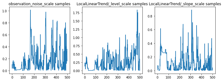
We can sanity-check the inference by examining the parameter traces. In this case they appear to have explored multiple explanations for the data, which is good, although more samples would be helpful to judge how well the chain is mixing.
f = plt.figure(figsize=(12, 4))
for i, param in enumerate(sts_model.parameters):
  ax = f.add_subplot(1, len(sts_model.parameters), i + 1)
  ax.plot(samples[i])
  ax.set_title("{} samples".format(param.name))
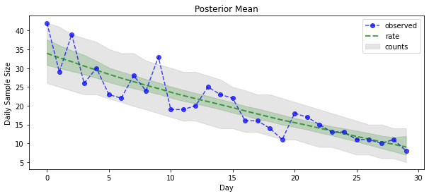
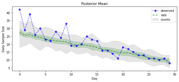
Now for the payoff: let's see the posterior over Poisson rates! We'll also plot the 80% predictive interval over observed counts, and can check that this interval appears to contain about 80% of the counts we actually observed.
param_samples = samples[:-1]
unconstrained_rate_samples = samples[-1][..., 0]
rate_samples = positive_bijector.forward(unconstrained_rate_samples)

plt.figure(figsize=(10, 4))
mean_lower, mean_upper = np.percentile(rate_samples, [10, 90], axis=0)
pred_lower, pred_upper = np.percentile(np.random.poisson(rate_samples),
                                       [10, 90], axis=0)

_ = plt.plot(observed_counts, color="blue", ls='--', marker='o', label='observed', alpha=0.7)
_ = plt.plot(np.mean(rate_samples, axis=0), label='rate', color="green", ls='dashed', lw=2, alpha=0.7)
_ = plt.fill_between(np.arange(0, 30), mean_lower, mean_upper, color='green', alpha=0.2)
_ = plt.fill_between(np.arange(0, 30), pred_lower, pred_upper, color='grey', label='counts', alpha=0.2)
plt.xlabel("Day")
plt.ylabel("Daily Sample Size")
plt.title("Posterior Mean")
plt.legend()
<matplotlib.legend.Legend at 0x7f93ffd35550>
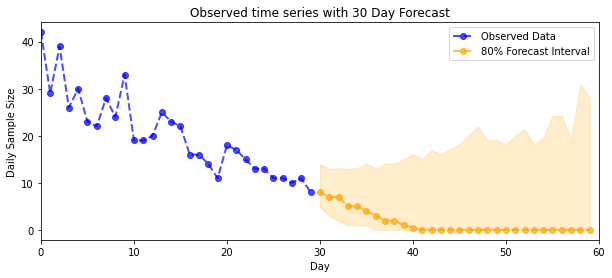
Forecasting
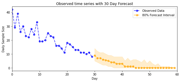
To forecast the observed counts, we'll use the standard STS tools to build a forecast distribution over the latent rates (in unconstrained space, again since STS is designed to model real-valued data), then pass the sampled forecasts through a Poisson observation model:
def sample_forecasted_counts(sts_model, posterior_latent_rates,
                             posterior_params, num_steps_forecast,
                             num_sampled_forecasts):

  # Forecast the future latent unconstrained rates, given the inferred latent
  # unconstrained rates and parameters.
  unconstrained_rates_forecast_dist = tfp.sts.forecast(sts_model,
    observed_time_series=unconstrained_rate_samples,
    parameter_samples=posterior_params,
    num_steps_forecast=num_steps_forecast)

  # Transform the forecast to positive-valued Poisson rates.
  rates_forecast_dist = tfd.TransformedDistribution(
      unconstrained_rates_forecast_dist,
      positive_bijector)

  # Sample from the forecast model following the chain rule:
  # P(counts) = P(counts | latent_rates)P(latent_rates)
  sampled_latent_rates = rates_forecast_dist.sample(num_sampled_forecasts)
  sampled_forecast_counts = tfd.Poisson(rate=sampled_latent_rates).sample()

  return sampled_forecast_counts, sampled_latent_rates

forecast_samples, rate_samples = sample_forecasted_counts(
   sts_model,
   posterior_latent_rates=unconstrained_rate_samples,
   posterior_params=param_samples,
   # Days to forecast:
   num_steps_forecast=30,
   num_sampled_forecasts=100)
forecast_samples = np.squeeze(forecast_samples)
def plot_forecast_helper(data, forecast_samples, CI=90):
  """Plot the observed time series alongside the forecast."""
  plt.figure(figsize=(10, 4))
  forecast_median = np.median(forecast_samples, axis=0)

  num_steps = len(data)
  num_steps_forecast = forecast_median.shape[-1]

  plt.plot(np.arange(num_steps), data, lw=2, color='blue', linestyle='--', marker='o',
           label='Observed Data', alpha=0.7)

  forecast_steps = np.arange(num_steps, num_steps+num_steps_forecast)

  CI_interval = [(100 - CI)/2, 100 - (100 - CI)/2]
  lower, upper = np.percentile(forecast_samples, CI_interval, axis=0)

  plt.plot(forecast_steps, forecast_median, lw=2, ls='--', marker='o', color='orange',
           label=str(CI) + '% Forecast Interval', alpha=0.7)
  plt.fill_between(forecast_steps,
                   lower,
                   upper, color='orange', alpha=0.2)

  plt.xlim([0, num_steps+num_steps_forecast])
  ymin, ymax = min(np.min(forecast_samples), np.min(data)), max(np.max(forecast_samples), np.max(data))
  yrange = ymax-ymin
  plt.title("{}".format('Observed time series with ' + str(num_steps_forecast) + ' Day Forecast'))
  plt.xlabel('Day')
  plt.ylabel('Daily Sample Size')
  plt.legend()
plot_forecast_helper(observed_counts, forecast_samples, CI=80)
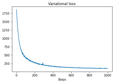
VI inference
Variational inference can be problematic when inferring a full time series, like our approximate counts (as opposed to just the parameters of a time series, as in standard STS models). The standard assumption that variables have independent posteriors is quite wrong, since each timestep is correlated with its neighbors, which can lead to underestimating uncertainty. For this reason, HMC may be a better choice for approximate inference over full time series. However, VI can be quite a bit faster, and may be useful for model prototyping or in cases where its performance can be empirically shown to be 'good enough'.
To fit our model with VI, we simply build and optimize a surrogate posterior:
surrogate_posterior = tfp.experimental.vi.build_factored_surrogate_posterior(
    event_shape=pinned_model.event_shape,
    bijector=constraining_bijector)
# Allow external control of optimization to reduce test runtimes.
num_variational_steps = 1000 # @param { isTemplate: true}
num_variational_steps = int(num_variational_steps)

t0 = time.time()
losses = tfp.vi.fit_surrogate_posterior(pinned_model.unnormalized_log_prob,
                                        surrogate_posterior,
                                        optimizer=tf_keras.optimizers.Adam(0.1),
                                        num_steps=num_variational_steps)
t1 = time.time()
print("Inference ran in {:.2f}s.".format(t1-t0))
Inference ran in 11.37s.
plt.plot(losses)
plt.title("Variational loss")
_ = plt.xlabel("Steps")
posterior_samples = surrogate_posterior.sample(50)
param_samples = posterior_samples[:-1]
unconstrained_rate_samples = posterior_samples[-1][..., 0]
rate_samples = positive_bijector.forward(unconstrained_rate_samples)

plt.figure(figsize=(10, 4))
mean_lower, mean_upper = np.percentile(rate_samples, [10, 90], axis=0)
pred_lower, pred_upper = np.percentile(
    np.random.poisson(rate_samples), [10, 90], axis=0)

_ = plt.plot(observed_counts, color='blue', ls='--', marker='o',
             label='observed', alpha=0.7)
_ = plt.plot(np.mean(rate_samples, axis=0), label='rate', color='green',
             ls='dashed', lw=2, alpha=0.7)
_ = plt.fill_between(
    np.arange(0, 30), mean_lower, mean_upper, color='green', alpha=0.2)
_ = plt.fill_between(np.arange(0, 30), pred_lower, pred_upper, color='grey',
    label='counts', alpha=0.2)
plt.xlabel('Day')
plt.ylabel('Daily Sample Size')
plt.title('Posterior Mean')
plt.legend()
<matplotlib.legend.Legend at 0x7f93ff4735c0>
forecast_samples, rate_samples = sample_forecasted_counts(
   sts_model,
   posterior_latent_rates=unconstrained_rate_samples,
   posterior_params=param_samples,
   # Days to forecast:
   num_steps_forecast=30,
   num_sampled_forecasts=100)
forecast_samples = np.squeeze(forecast_samples)
plot_forecast_helper(observed_counts, forecast_samples, CI=80)