TensorFlow กลับมาที่ Google I/O ในวันที่ 14 พฤษภาคม! สมัครตอนนี้

หน้านี้ได้รับการแปลโดย Cloud Translation API

การแสดงข้อมูลภาพใน TensorBoard

ดูบน TensorFlow.org

ทำงานใน Google Colab

ดูแหล่งที่มาบน GitHub

ดาวน์โหลดโน๊ตบุ๊ค

ภาพรวม

ใช้ TensorFlow ภาพอย่างย่อ API คุณสามารถเข้าสู่ระบบเทนเซอร์และภาพโดยพลการและดูพวกเขาใน TensorBoard ซึ่งจะเป็นประโยชน์อย่างยิ่งที่จะได้ลิ้มลองและตรวจสอบการป้อนข้อมูลของคุณหรือ เห็นภาพน้ำหนักชั้น และ เทนเซอร์ที่สร้าง คุณยังสามารถบันทึกข้อมูลการวินิจฉัยเป็นอิมเมจที่เป็นประโยชน์ในระหว่างการพัฒนาแบบจำลองของคุณ

ในบทช่วยสอนนี้ คุณจะได้เรียนรู้วิธีใช้ Image Summary API เพื่อแสดงภาพเทนเซอร์เป็นรูปภาพ คุณจะได้เรียนรู้วิธีถ่ายภาพตามอำเภอใจ แปลงเป็นเทนเซอร์ และแสดงภาพใน TensorBoard คุณจะทำงานผ่านตัวอย่างที่เรียบง่ายแต่มีอยู่จริงซึ่งใช้ Image Summaries เพื่อช่วยให้คุณเข้าใจว่าแบบจำลองของคุณทำงานเป็นอย่างไร

ติดตั้ง

try:
  # %tensorflow_version only exists in Colab.
  %tensorflow_version 2.x
except Exception:
  pass

# Load the TensorBoard notebook extension.
%load_ext tensorboard

TensorFlow 2.x selected.

from datetime import datetime
import io
import itertools
from packaging import version

import tensorflow as tf
from tensorflow import keras

import matplotlib.pyplot as plt
import numpy as np
import sklearn.metrics

print("TensorFlow version: ", tf.__version__)
assert version.parse(tf.__version__).release[0] >= 2, \
    "This notebook requires TensorFlow 2.0 or above."

TensorFlow version:  2.2

ดาวน์โหลดชุดข้อมูล Fashion-MNIST

คุณจะสร้างเครือข่ายประสาทง่ายต่อการแยกประเภทภาพในที่ แฟชั่น MNIST ชุด ชุดข้อมูลนี้ประกอบด้วยรูปภาพระดับสีเทาขนาด 28x28 70,000 ของผลิตภัณฑ์แฟชั่นจาก 10 หมวดหมู่ โดยมี 7,000 ภาพต่อหมวดหมู่

ขั้นแรก ดาวน์โหลดข้อมูล:

# Download the data. The data is already divided into train and test.
# The labels are integers representing classes.
fashion_mnist = keras.datasets.fashion_mnist
(train_images, train_labels), (test_images, test_labels) = \
    fashion_mnist.load_data()

# Names of the integer classes, i.e., 0 -> T-short/top, 1 -> Trouser, etc.
class_names = ['T-shirt/top', 'Trouser', 'Pullover', 'Dress', 'Coat', 
    'Sandal', 'Shirt', 'Sneaker', 'Bag', 'Ankle boot']

Downloading data from https://storage.googleapis.com/tensorflow/tf-keras-datasets/train-labels-idx1-ubyte.gz
32768/29515 [=================================] - 0s 0us/step
Downloading data from https://storage.googleapis.com/tensorflow/tf-keras-datasets/train-images-idx3-ubyte.gz
26427392/26421880 [==============================] - 0s 0us/step
Downloading data from https://storage.googleapis.com/tensorflow/tf-keras-datasets/t10k-labels-idx1-ubyte.gz
8192/5148 [===============================================] - 0s 0us/step
Downloading data from https://storage.googleapis.com/tensorflow/tf-keras-datasets/t10k-images-idx3-ubyte.gz
4423680/4422102 [==============================] - 0s 0us/step

การแสดงภาพเดียว

เพื่อให้เข้าใจว่า Image Summary API ทำงานอย่างไร ตอนนี้คุณจะต้องบันทึกอิมเมจการฝึกแรกในชุดการฝึกของคุณใน TensorBoard

ก่อนที่คุณจะทำเช่นนั้น ให้ตรวจสอบรูปร่างของข้อมูลการฝึกของคุณ:

print("Shape: ", train_images[0].shape)
print("Label: ", train_labels[0], "->", class_names[train_labels[0]])

Shape:  (28, 28)
Label:  9 -> Ankle boot

สังเกตว่ารูปร่างของแต่ละภาพในชุดข้อมูลเป็นเทนเซอร์ของรูปร่างอันดับ 2 (28, 28) ซึ่งแสดงถึงความสูงและความกว้าง

อย่างไรก็ตาม tf.summary.image() คาดว่าจะมีการจัดอันดับ-4 เมตริกซ์ที่มี (batch_size, height, width, channels) ดังนั้นเทนเซอร์จึงต้องเปลี่ยนรูปใหม่

คุณเข้าสู่ระบบเป็นเพียงภาพหนึ่งดังนั้น batch_size คือ 1. ภาพที่มีสีเทา, ตั้งค่าเพื่อให้ channels 1

# Reshape the image for the Summary API.
img = np.reshape(train_images[0], (-1, 28, 28, 1))

ตอนนี้คุณพร้อมที่จะบันทึกภาพนี้และดูใน TensorBoard แล้ว

# Clear out any prior log data.
!rm -rf logs

# Sets up a timestamped log directory.
logdir = "logs/train_data/" + datetime.now().strftime("%Y%m%d-%H%M%S")
# Creates a file writer for the log directory.
file_writer = tf.summary.create_file_writer(logdir)

# Using the file writer, log the reshaped image.
with file_writer.as_default():
  tf.summary.image("Training data", img, step=0)

ตอนนี้ ใช้ TensorBoard เพื่อตรวจสอบรูปภาพ รอสักครู่เพื่อให้ UI หมุน

%tensorboard --logdir logs/train_data

แท็บ "รูปภาพ" จะแสดงรูปภาพที่คุณเพิ่งเข้าสู่ระบบ มันคือ "รองเท้าบูทหุ้มข้อ"

รูปภาพถูกปรับขนาดเป็นขนาดเริ่มต้นเพื่อให้ดูได้ง่ายขึ้น หากคุณต้องการดูภาพต้นฉบับที่ไม่ได้ปรับขนาด ให้เลือก "แสดงขนาดภาพจริง" ที่ด้านบนซ้าย

เล่นกับแถบเลื่อนความสว่างและความคมชัดเพื่อดูว่ามีผลต่อพิกเซลของภาพอย่างไร

การแสดงภาพหลายภาพ

การบันทึกหนึ่งเทนเซอร์นั้นยอดเยี่ยม แต่ถ้าคุณต้องการบันทึกตัวอย่างการฝึกหลายๆ ตัวอย่างล่ะ

เพียงแค่ระบุจำนวนภาพที่คุณต้องการเข้าสู่ระบบเมื่อผ่านข้อมูลไปยัง tf.summary.image()

with file_writer.as_default():
  # Don't forget to reshape.
  images = np.reshape(train_images[0:25], (-1, 28, 28, 1))
  tf.summary.image("25 training data examples", images, max_outputs=25, step=0)

%tensorboard --logdir logs/train_data

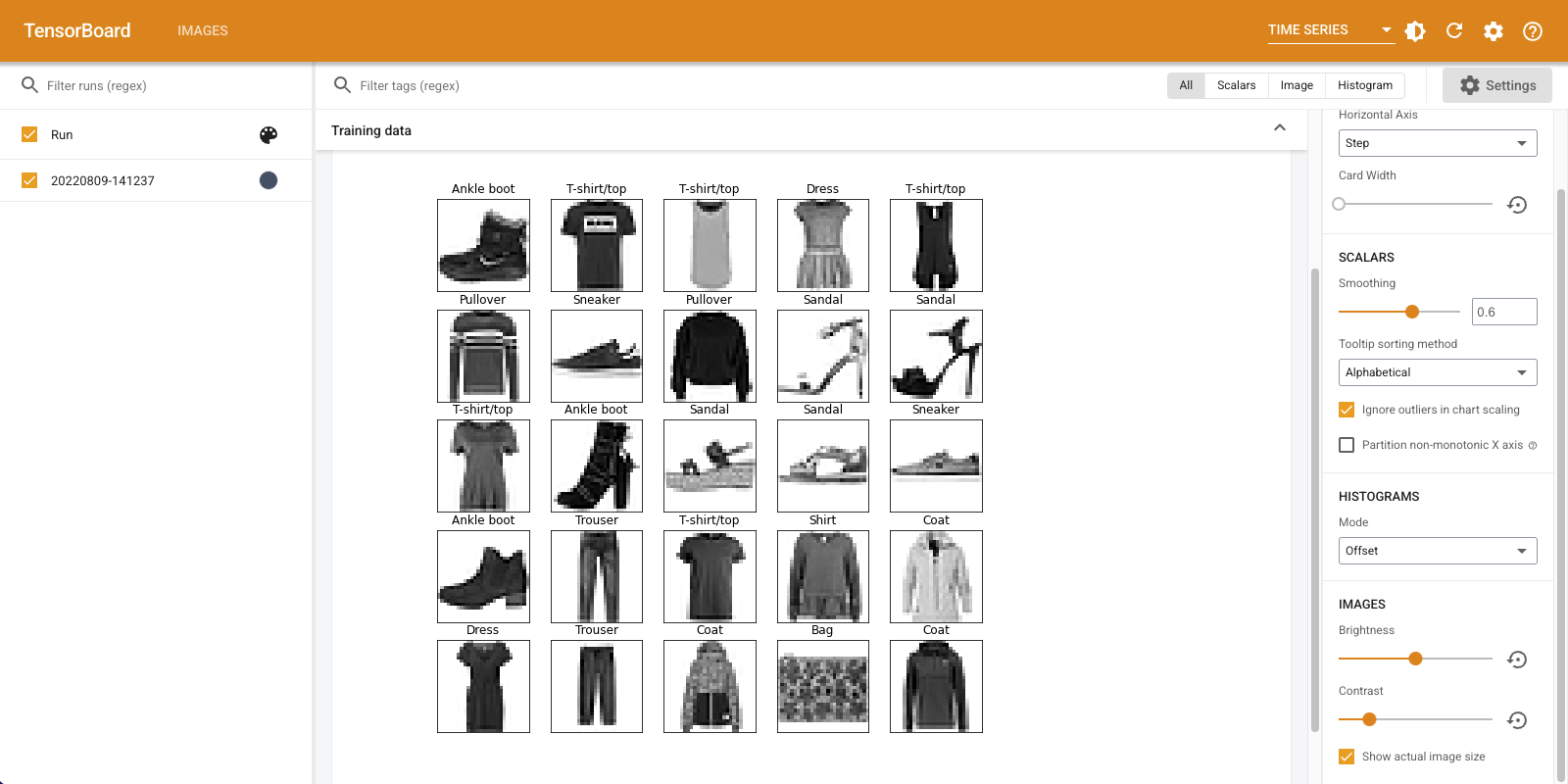
กำลังบันทึกข้อมูลภาพโดยพลการ

ถ้าคุณต้องการที่จะเห็นภาพภาพที่ไม่เมตริกซ์เช่นภาพที่สร้างขึ้นโดย matplotlib ?

คุณต้องมีรหัสสำเร็จรูปเพื่อแปลงพล็อตเป็นเทนเซอร์ แต่หลังจากนั้น คุณก็พร้อมแล้ว

ในรหัสข้างล่างนี้คุณจะเข้าสู่ระบบ 25 ภาพแรกเป็นตารางที่ดีโดยใช้ matplotlib ของ subplot() ฟังก์ชั่น จากนั้นคุณจะดูตารางใน TensorBoard:

# Clear out prior logging data.
!rm -rf logs/plots

logdir = "logs/plots/" + datetime.now().strftime("%Y%m%d-%H%M%S")
file_writer = tf.summary.create_file_writer(logdir)

def plot_to_image(figure):
  """Converts the matplotlib plot specified by 'figure' to a PNG image and
  returns it. The supplied figure is closed and inaccessible after this call."""
  # Save the plot to a PNG in memory.
  buf = io.BytesIO()
  plt.savefig(buf, format='png')
  # Closing the figure prevents it from being displayed directly inside
  # the notebook.
  plt.close(figure)
  buf.seek(0)
  # Convert PNG buffer to TF image
  image = tf.image.decode_png(buf.getvalue(), channels=4)
  # Add the batch dimension
  image = tf.expand_dims(image, 0)
  return image

def image_grid():
  """Return a 5x5 grid of the MNIST images as a matplotlib figure."""
  # Create a figure to contain the plot.
  figure = plt.figure(figsize=(10,10))
  for i in range(25):
    # Start next subplot.
    plt.subplot(5, 5, i + 1, title=class_names[train_labels[i]])
    plt.xticks([])
    plt.yticks([])
    plt.grid(False)
    plt.imshow(train_images[i], cmap=plt.cm.binary)

  return figure

# Prepare the plot
figure = image_grid()
# Convert to image and log
with file_writer.as_default():
  tf.summary.image("Training data", plot_to_image(figure), step=0)

%tensorboard --logdir logs/plots

การสร้างตัวแยกประเภทภาพ

ตอนนี้นำทั้งหมดนี้มารวมกันด้วยตัวอย่างที่แท้จริง เพราะคุณมาที่นี่เพื่อทำการเรียนรู้ด้วยเครื่องและไม่ได้สร้างภาพที่สวยงามแต่อย่างใด!

คุณจะใช้การสรุปรูปภาพเพื่อทำความเข้าใจว่าโมเดลของคุณทำงานได้ดีเพียงใดในขณะที่ฝึกตัวแยกประเภทอย่างง่ายสำหรับชุดข้อมูล Fashion-MNIST

ขั้นแรก สร้างโมเดลที่ง่ายมากและคอมไพล์ ตั้งค่าตัวเพิ่มประสิทธิภาพและฟังก์ชันการสูญเสีย ขั้นตอนการคอมไพล์ยังระบุว่าคุณต้องการบันทึกความถูกต้องของตัวแยกประเภทไปพร้อมกัน

model = keras.models.Sequential([
    keras.layers.Flatten(input_shape=(28, 28)),
    keras.layers.Dense(32, activation='relu'),
    keras.layers.Dense(10, activation='softmax')
])

model.compile(
    optimizer='adam', 
    loss='sparse_categorical_crossentropy',
    metrics=['accuracy']
)

เมื่อการฝึกอบรมลักษณนามก็มีประโยชน์ที่จะเห็น เมทริกซ์ความสับสน เมทริกซ์ความสับสนช่วยให้คุณทราบรายละเอียดว่าตัวแยกประเภทของคุณทำงานอย่างไรกับข้อมูลการทดสอบ

กำหนดฟังก์ชันที่คำนวณเมทริกซ์ความสับสน คุณจะใช้ความสะดวกสบาย Scikit เรียนรู้ ฟังก์ชั่นการทำเช่นนี้แล้วพล็อตโดยใช้ matplotlib

def plot_confusion_matrix(cm, class_names):
  """
  Returns a matplotlib figure containing the plotted confusion matrix.

  Args:
    cm (array, shape = [n, n]): a confusion matrix of integer classes
    class_names (array, shape = [n]): String names of the integer classes
  """
  figure = plt.figure(figsize=(8, 8))
  plt.imshow(cm, interpolation='nearest', cmap=plt.cm.Blues)
  plt.title("Confusion matrix")
  plt.colorbar()
  tick_marks = np.arange(len(class_names))
  plt.xticks(tick_marks, class_names, rotation=45)
  plt.yticks(tick_marks, class_names)

  # Compute the labels from the normalized confusion matrix.
  labels = np.around(cm.astype('float') / cm.sum(axis=1)[:, np.newaxis], decimals=2)

  # Use white text if squares are dark; otherwise black.
  threshold = cm.max() / 2.
  for i, j in itertools.product(range(cm.shape[0]), range(cm.shape[1])):
    color = "white" if cm[i, j] > threshold else "black"
    plt.text(j, i, labels[i, j], horizontalalignment="center", color=color)

  plt.tight_layout()
  plt.ylabel('True label')
  plt.xlabel('Predicted label')
  return figure

ตอนนี้คุณพร้อมที่จะฝึกลักษณนามและบันทึกเมทริกซ์ความสับสนตลอดเส้นทางแล้ว

นี่คือสิ่งที่คุณจะทำ:

สร้าง การเรียกกลับ Keras TensorBoard เข้าสู่ระบบเมตริกพื้นฐาน
สร้าง Keras LambdaCallback เข้าสู่ระบบเมทริกซ์ความสับสนในตอนท้ายของทุกยุค
ฝึกโมเดลโดยใช้ Model.fit() ตรวจสอบให้แน่ใจว่าผ่านการเรียกกลับทั้งคู่

ขณะที่การฝึกดำเนินไป ให้เลื่อนลงเพื่อดู TensorBoard ที่เริ่มทำงาน

# Clear out prior logging data.
!rm -rf logs/image

logdir = "logs/image/" + datetime.now().strftime("%Y%m%d-%H%M%S")
# Define the basic TensorBoard callback.
tensorboard_callback = keras.callbacks.TensorBoard(log_dir=logdir)
file_writer_cm = tf.summary.create_file_writer(logdir + '/cm')

def log_confusion_matrix(epoch, logs):
  # Use the model to predict the values from the validation dataset.
  test_pred_raw = model.predict(test_images)
  test_pred = np.argmax(test_pred_raw, axis=1)

  # Calculate the confusion matrix.
  cm = sklearn.metrics.confusion_matrix(test_labels, test_pred)
  # Log the confusion matrix as an image summary.
  figure = plot_confusion_matrix(cm, class_names=class_names)
  cm_image = plot_to_image(figure)

  # Log the confusion matrix as an image summary.
  with file_writer_cm.as_default():
    tf.summary.image("Confusion Matrix", cm_image, step=epoch)

# Define the per-epoch callback.
cm_callback = keras.callbacks.LambdaCallback(on_epoch_end=log_confusion_matrix)

# Start TensorBoard.
%tensorboard --logdir logs/image

# Train the classifier.
model.fit(
    train_images,
    train_labels,
    epochs=5,
    verbose=0, # Suppress chatty output
    callbacks=[tensorboard_callback, cm_callback],
    validation_data=(test_images, test_labels),
)

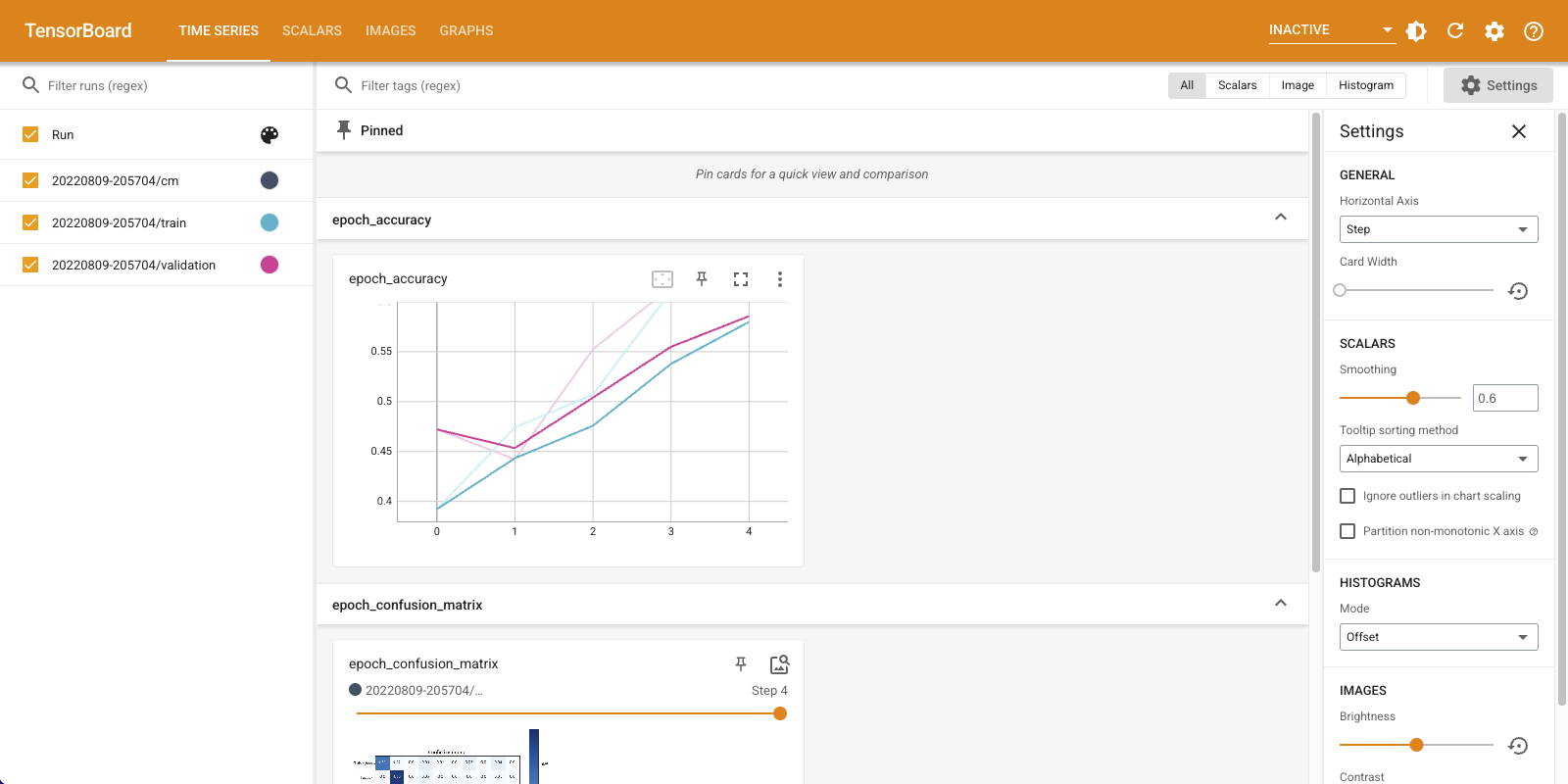
ขอให้สังเกตว่าความแม่นยำกำลังเพิ่มขึ้นทั้งบนรถไฟและชุดตรวจสอบ นั่นเป็นสัญญาณที่ดี แต่โมเดลทำงานอย่างไรกับชุดย่อยเฉพาะของข้อมูล

เลือกแท็บ "รูปภาพ" เพื่อแสดงภาพเมทริกซ์ความสับสนที่บันทึกไว้ของคุณ ทำเครื่องหมายที่ "แสดงขนาดภาพจริง" ที่ด้านบนซ้ายเพื่อดูเมทริกซ์ความสับสนในขนาดเต็ม

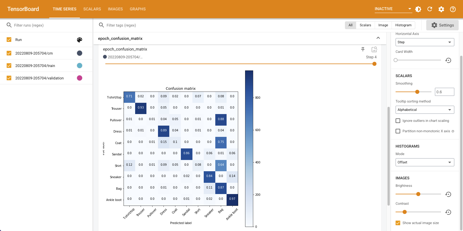
โดยค่าเริ่มต้น แดชบอร์ดจะแสดงภาพสรุปสำหรับขั้นตอนหรือยุคที่บันทึกล่าสุด ใช้แถบเลื่อนเพื่อดูเมทริกซ์ความสับสนก่อนหน้า สังเกตว่าเมทริกซ์เปลี่ยนแปลงอย่างมีนัยสำคัญเมื่อการฝึกดำเนินไปอย่างไร โดยสี่เหลี่ยมสีเข้มจะรวมกันตามแนวทแยง และเมทริกซ์ที่เหลือจะพุ่งเข้าหา 0 และสีขาว ซึ่งหมายความว่าลักษณนามของคุณพัฒนาขึ้นเมื่อการฝึกอบรมดำเนินไป! การทำงานที่ดี!

เมทริกซ์ความสับสนแสดงให้เห็นว่าโมเดลอย่างง่ายนี้มีปัญหาบางอย่าง แม้จะมีความคืบหน้าอย่างมาก เสื้อเชิ้ต เสื้อยืด และเสื้อสวมหัวก็กำลังสับสนซึ่งกันและกัน แบบจำลองต้องการการทำงานมากขึ้น

หากคุณสนใจ, พยายามที่จะปรับปรุงรูปแบบนี้มี เครือข่ายความสับสน (ซีเอ็นเอ็น)