
| |
|
 在 GitHub 上查看源代码 在 GitHub 上查看源代码 |
|
变分推断 (VI) 将近似贝叶斯推断转换为一个优化问题,并寻求一个“代理”后验分布,以尽可能减小与真实后验的 KL 散度。基于梯度的 VI 通常比 MCMC 方法更快,与模型参数的优化自然组合,并提供模型证据的下界,可直接用于模型比较、收敛诊断和组合式推断。
TensorFlow Probability 为快速、灵活和可扩展的 VI 提供了可自然适合 TFP 堆栈的工具。通过这些工具可以构造具有由线性变换或归一化流引入的协方差结构的代理后验。
VI 可以用于估计回归模型参数的贝叶斯可信区间,以估计各种处理或观察到的特征对感兴趣结果的影响。可信区间根据以观测数据为条件的参数的后验分布,并考虑到对参数先验分布的假设,以一定的概率约束未观测到的参数的值。
在本 Colab 中,我们将演示如何使用 VI 来获得在家中测量的氡水平的贝叶斯线性回归模型参数的可信区间(使用 Gelman 等人 (2007) 的氡数据集;请参见 Stan 中的类似示例)。我们将演示 TFP JointDistribution 如何与 bijectors 相结合,来构建和拟合两种类型的表达代理后验:
- 由块矩阵变换的标准正态分布。该矩阵可以反映后验的某些成分之间的独立性和其他成分之间的依赖关系,从而放宽平均场或全协方差后验的假设。
- 更复杂、容量更大的逆自回归流。
代理后验经过训练后,与平均场代理后验基线的结果以及哈密顿蒙特卡洛的真实样本进行比较。
贝叶斯变分推断概述
假设我们有以下生成过程,其中 \(\theta\) 表示随机参数,\(\omega\) 表示确定性参数,\(x_i\) 是特征,\(y_i\) 是 \(i=1,\ldots,n\) 观测的数据点的目标值:\begin{align} &\theta \sim r(\Theta) && \text{(Prior)}\ &\text{for } i = 1 \ldots n: \nonumber \ &\quad y_i \sim p(Y_i|x_i, \theta, \omega) && \text{(Likelihood)} \end{align}
然后,VI 的特征为:\(\newcommand{\E}{\operatorname{\mathbb{E} } } \newcommand{\K}{\operatorname{\mathbb{K} } } \newcommand{\defeq}{\overset{\tiny\text{def} }{=} } \DeclareMathOperator*{\argmin}{arg,min}\)
\begin{align} -\log p({y_i}_i^n|{x_i}i^n, \omega) &\defeq -\log \int \textrm{d}\theta, r(\theta) \prod_i^n p(y_i|x_i,\theta, \omega) && \text{(Really hard integral)} \ &= -\log \int \textrm{d}\theta, q(\theta) \frac{1}{q(\theta)} r(\theta) \prod_i^n p(y_i|x_i,\theta, \omega) && \text{(Multiply by 1)}\ &\le - \int \textrm{d}\theta, q(\theta) \log \frac{r(\theta) \prod_i^n p(y_i|x_i,\theta, \omega)}{q(\theta)} && \text{(Jensen's inequality)}\ &\defeq \E{q(\Theta)}[ -\log p(y_i|x_i,\Theta, \omega) ] + \K[q(\Theta), r(\Theta)]\ &\defeq \text{expected negative log likelihood"} +\text{kl regularizer"} \end{align}
(技术上,我们假定 \(q\) 相对于 \(r\) 是绝对连续的。另请参阅詹森不等式。)
由于边界对所有 q 都成立,显然对于以下公式是最紧的:
\[q^*,w^* = \argmin_{q \in \mathcal{Q},\omega\in\mathbb{R}^d} \left{ \sum_i^n\E_{q(\Theta)}\left[ -\log p(y_i|x_i,\Theta, \omega) \right] + \K[q(\Theta), r(\Theta)] \right}\]
在术语方面,我们将
- \(q^*\) 称为“代理后验”,
- \(\mathcal{Q}\) 称为“代理家族”。
\(\omega^*\) 表示 VI 损失的确定性参数的最大似然值。有关变分推断的更多信息,请参阅此调查。
示例:氡测量值的贝叶斯分层线性回归
氡是一种放射性气体,它通过与地面的接触点进入房屋。它是一种致癌物质,是非吸烟者患上肺癌的主要原因。不同房屋的氡水平差异很大。
环保署对 80,000 所房屋中的氡水平进行了研究。两个重要的预测指标是:
- 进行测量的楼层(地下室的氡含量较高)
- 县的铀水平(与氡水平正相关)
预测按县分组的房屋中的氡水平是贝叶斯分层建模的一个经典问题,由 Gelman 和 Hill (2006) 提出。我们将建立一个分层线性模型来预测房屋中的氡测量值,其中的层级结构是按县对房屋进行的分组。我们对明尼苏达州的房屋位置(县)对氡水平的影响的可信区间感兴趣。为了隔离这种影响,楼层和铀水平的影响也包括在模型中。此外,我们还将引入一个按县区分的环境效应,对应于进行测量的平均楼层,这样,如果进行测量的楼层所在的县之间存在差异,则不归因于县效应。
pip3 install -q tf-nightly tfp-nightlyimport matplotlib.pyplot as plt
import numpy as np
import seaborn as sns
import tensorflow as tf
import tensorflow_datasets as tfds
import tensorflow_probability as tfp
import warnings
tfd = tfp.distributions
tfb = tfp.bijectors
plt.rcParams['figure.facecolor'] = '1.'
# Load the Radon dataset from `tensorflow_datasets` and filter to data from
# Minnesota.
dataset = tfds.as_numpy(
    tfds.load('radon', split='train').filter(
        lambda x: x['features']['state'] == 'MN').batch(10**9))

# Dependent variable: Radon measurements by house.
dataset = next(iter(dataset))
radon_measurement = dataset['activity'].astype(np.float32)
radon_measurement[radon_measurement <= 0.] = 0.1
log_radon = np.log(radon_measurement)

# Measured uranium concentrations in surrounding soil.
uranium_measurement = dataset['features']['Uppm'].astype(np.float32)
log_uranium = np.log(uranium_measurement)

# County indicator.
county_strings = dataset['features']['county'].astype('U13')
unique_counties, county = np.unique(county_strings, return_inverse=True)
county = county.astype(np.int32)
num_counties = unique_counties.size

# Floor on which the measurement was taken.
floor_of_house = dataset['features']['floor'].astype(np.int32)

# Average floor by county (contextual effect).
county_mean_floor = []
for i in range(num_counties):
  county_mean_floor.append(floor_of_house[county == i].mean())
county_mean_floor = np.array(county_mean_floor, dtype=log_radon.dtype)
floor_by_county = county_mean_floor[county]
该回归模型指定如下:
\(\newcommand{\Normal}{\operatorname{\sf Normal} }\) \begin{align} &\text{uranium_weight} \sim \Normal(0, 1) \ &\text{county_floor_weight} \sim \Normal(0, 1) \ &\text{for } j = 1\ldots \text{num_counties}:\ &\quad \text{county_effect}j \sim \Normal (0, \sigma_c)\ &\text{for } i = 1\ldots n:\ &\quad \mu_i = ( \ &\quad\quad \text{bias} \ &\quad\quad + \text{county_effect}{\text{county}_i} \ &\quad\quad +\text{log_uranium}_i \times \text{uranium_weight} \ &\quad\quad +\text{floor_of_house}i \times \text{floor_weight} \ &\quad\quad +\text{floor_by_county}{\text{county}_i} \times \text{county_floor_weight} ) \ &\quad \text{log_radon}_i \sim \Normal(\mu_i, \sigma_y) \end{align},其中 \(i\) 是观测值的索引,\(\text{county}_i\) 是进行第 \(i\) 次测量时所在的县。
我们使用县级随机影响来捕捉地理差异。参数 uranium_weight 和 county_floor_weight 是概率建模的,而 floor_weight 和常量 bias 是确定性的。这些建模选择在很大程度上是任意的,目的是在具有合理复杂性的概率模型上演示 VI。有关使用氡数据集在 TFP 中进行具有固定和随机影响的多级建模的更全面讨论,请参阅多级建模入门和使用变分推断拟合广义线性混合效应模型 。
# Create variables for fixed effects.
floor_weight = tf.Variable(0.)
bias = tf.Variable(0.)

# Variables for scale parameters.
log_radon_scale = tfp.util.TransformedVariable(1., tfb.Exp())
county_effect_scale = tfp.util.TransformedVariable(1., tfb.Exp())

# Define the probabilistic graphical model as a JointDistribution.
@tfd.JointDistributionCoroutineAutoBatched
def model():
  uranium_weight = yield tfd.Normal(0., scale=1., name='uranium_weight')
  county_floor_weight = yield tfd.Normal(
      0., scale=1., name='county_floor_weight')
  county_effect = yield tfd.Sample(
      tfd.Normal(0., scale=county_effect_scale),
      sample_shape=[num_counties], name='county_effect')
  yield tfd.Normal(
      loc=(log_uranium * uranium_weight + floor_of_house* floor_weight
           + floor_by_county * county_floor_weight
           + tf.gather(county_effect, county, axis=-1)
           + bias),
      scale=log_radon_scale[..., tf.newaxis],
      name='log_radon')

# Pin the observed `log_radon` values to model the un-normalized posterior.
target_model = model.experimental_pin(log_radon=log_radon)
表达代理后验
接下来,我们使用具有两种不同类型的代理后验的 VI 来估计随机影响的后验分布:
- 受约束的多元正态分布,具有由分块矩阵变换引起的协方差结构。
- 多元标准正态分布,由逆自回归流变换而来,然后进行拆分和重组以匹配后验的支持。
多元正态代理后验
为了构建该代理后验,使用可训练的线性算子来诱导后验成分之间的相关性。
# Determine the `event_shape` of the posterior, and calculate the size of each
# `event_shape` component. These determine the sizes of the components of the
# underlying standard Normal distribution, and the dimensions of the blocks in
# the blockwise matrix transformation.
event_shape = target_model.event_shape_tensor()
flat_event_shape = tf.nest.flatten(event_shape)
flat_event_size = tf.nest.map_structure(tf.reduce_prod, flat_event_shape)

# The `event_space_bijector` maps unconstrained values (in R^n) to the support
# of the prior -- we'll need this at the end to constrain Multivariate Normal
# samples to the prior's support.
event_space_bijector = target_model.experimental_default_event_space_bijector()
构造一个具有向量值标准正态成分的 JointDistribution,大小由相应的先验成分确定。这些成分应该是向量值的,以便可以通过线性算子进行变换。
base_standard_dist = tfd.JointDistributionSequential(
      [tfd.Sample(tfd.Normal(0., 1.), s) for s in flat_event_size])
构建可训练的分块下三角线性算子。我们将其应用于标准正态分布以实现(可训练的)分块矩阵变换并诱导后验的相关结构。
在分块线性算子内,可训练的全矩阵块表示后验的两个分量之间的完全协方差,而由零组成的块(或 None)表示独立性。对角线上的块为下三角矩阵或对角矩阵,因此整个块结构表示一个下三角矩阵。
将此双射函数应用于基本分布会产生一个多元正态分布,其均值为 0,(Cholesky 因子)协方差等于下三角块矩阵。
operators = (
    (tf.linalg.LinearOperatorDiag,),  # Variance of uranium weight (scalar).
    (tf.linalg.LinearOperatorFullMatrix,  # Covariance between uranium and floor-by-county weights.
     tf.linalg.LinearOperatorDiag),  # Variance of floor-by-county weight (scalar).
    (None,  # Independence between uranium weight and county effects.
     None,  #  Independence between floor-by-county and county effects.
     tf.linalg.LinearOperatorDiag)  # Independence among the 85 county effects.
    )

block_tril_linop = (
    tfp.experimental.vi.util.build_trainable_linear_operator_block(
        operators, flat_event_size))
scale_bijector = tfb.ScaleMatvecLinearOperatorBlock(block_tril_linop)
将该线性算子应用于标准正态分布后,应用多部分 Shift 双射函数以允许均值取非零值。
loc_bijector = tfb.JointMap(
    tf.nest.map_structure(
        lambda s: tfb.Shift(
            tf.Variable(tf.random.uniform(
                (s,), minval=-2., maxval=2., dtype=tf.float32))),
        flat_event_size))
产生的多元正态分布(通过使用尺度和位置双射参数对标准正态分布进行变换获得)必须经过重塑和重构才能匹配先验,并最终受到先验支持的约束。
# Reshape each component to match the prior, using a nested structure of
# `Reshape` bijectors wrapped in `JointMap` to form a multipart bijector.
reshape_bijector = tfb.JointMap(
    tf.nest.map_structure(tfb.Reshape, flat_event_shape))

# Restructure the flat list of components to match the prior's structure
unflatten_bijector = tfb.Restructure(
        tf.nest.pack_sequence_as(
            event_shape, range(len(flat_event_shape))))
现在进行汇总 -- 将可训练的双射函数链接在一起,并将它们应用于基本标准正态分布以构造代理后验。
surrogate_posterior = tfd.TransformedDistribution(
    base_standard_dist,
    bijector = tfb.Chain(  # Note that the chained bijectors are applied in reverse order
        [
         event_space_bijector,  # constrain the surrogate to the support of the prior
         unflatten_bijector,  # pack the reshaped components into the `event_shape` structure of the posterior
         reshape_bijector,  # reshape the vector-valued components to match the shapes of the posterior components
         loc_bijector,  # allow for nonzero mean
         scale_bijector  # apply the block matrix transformation to the standard Normal distribution
         ]))
训练多元正态代理后验。
optimizer = tf.optimizers.Adam(learning_rate=1e-2)
mvn_loss = tfp.vi.fit_surrogate_posterior(
target_model.unnormalized_log_prob,
surrogate_posterior,
optimizer=optimizer,
num_steps=10**4,
sample_size=16,
jit_compile=True)
mvn_samples = surrogate_posterior.sample(1000)
mvn_final_elbo = tf.reduce_mean(
target_model.unnormalized_log_prob(*mvn_samples)
- surrogate_posterior.log_prob(mvn_samples))
print('Multivariate Normal surrogate posterior ELBO: {}'.format(mvn_final_elbo))
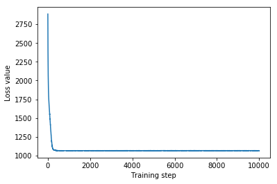
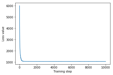
plt.plot(mvn_loss)
plt.xlabel('Training step')
_ = plt.ylabel('Loss value')
Multivariate Normal surrogate posterior ELBO: -1065.705322265625
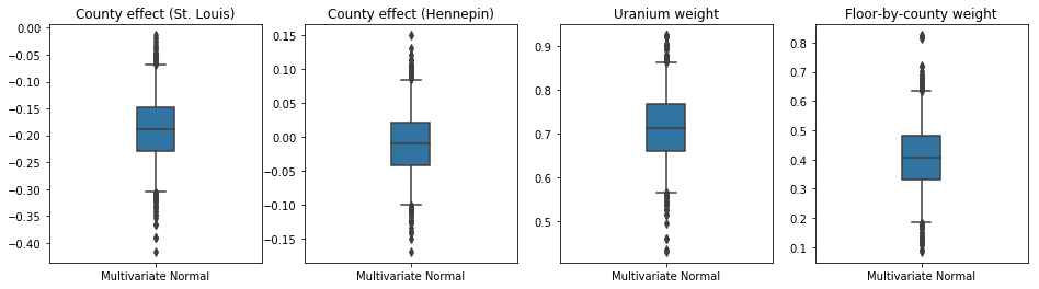
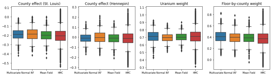
由于训练后的代理后验是 TFP 分布,我们可以从中抽取样本并对其进行处理,以生成参数的后验可信区间。
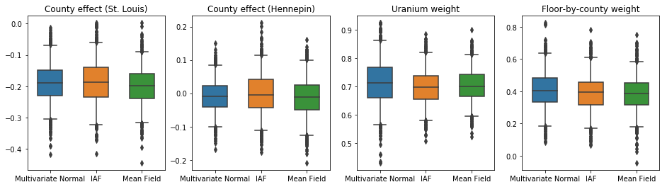
下面的盒须图显示了两个最大县的县效应以及土壤铀测量值和县平均楼层的回归权重的 50% 和 95% 可信区间。县效应的后验可信区间表明,在考虑其他变量后,圣路易斯县的位置与较低的氡水平相关,而亨内平县的位置效应接近中性。
回归权重的后验可信区间表明,土壤铀水平越高,氡水平越高,而在较高楼层进行测量的县(可能是因为房屋没有地下室)往往具有较高的氡水平,这可能与土壤特性及其对建筑结构类型的影响有关。
楼层的(确定性)系数为负,表明楼层越低,氡水平越高,正如预期。
st_louis_co = 69  # Index of St. Louis, the county with the most observations.
hennepin_co = 25  # Index of Hennepin, with the second-most observations.

def pack_samples(samples):
  return {'County effect (St. Louis)': samples.county_effect[..., st_louis_co],
          'County effect (Hennepin)': samples.county_effect[..., hennepin_co],
          'Uranium weight': samples.uranium_weight,
          'Floor-by-county weight': samples.county_floor_weight}

def plot_boxplot(posterior_samples):
  fig, axes = plt.subplots(1, 4, figsize=(16, 4))

  # Invert the results dict for easier plotting.
  k = list(posterior_samples.values())[0].keys()
  plot_results = {
      v: {p: posterior_samples[p][v] for p in posterior_samples} for v in k}
  for i, (var, var_results) in enumerate(plot_results.items()):
    sns.boxplot(data=list(var_results.values()), ax=axes[i],
                width=0.18*len(var_results), whis=(2.5, 97.5))
    # axes[i].boxplot(list(var_results.values()), whis=(2.5, 97.5))
    axes[i].title.set_text(var)
    fs = 10 if len(var_results) < 4 else 8
    axes[i].set_xticklabels(list(var_results.keys()), fontsize=fs)

results = {'Multivariate Normal': pack_samples(mvn_samples)}

print('Bias is: {:.2f}'.format(bias.numpy()))
print('Floor fixed effect is: {:.2f}'.format(floor_weight.numpy()))
plot_boxplot(results)
Bias is: 1.40
Floor fixed effect is: -0.72
逆自回归流代理后验
逆自回归流 (IAF) 是归一化流,使用神经网络来捕获分布成分之间的复杂、非线性依赖关系。接下来,我们将构建一个 IAF 代理后验,来看看这个容量更大、更灵活的模型是否优于受约束的多元正态模型。
# Build a standard Normal with a vector `event_shape`, with length equal to the
# total number of degrees of freedom in the posterior.
base_distribution = tfd.Sample(
    tfd.Normal(0., 1.), sample_shape=[tf.reduce_sum(flat_event_size)])

# Apply an IAF to the base distribution.
num_iafs = 2
iaf_bijectors = [
    tfb.Invert(tfb.MaskedAutoregressiveFlow(
        shift_and_log_scale_fn=tfb.AutoregressiveNetwork(
            params=2, hidden_units=[256, 256], activation='relu')))
    for _ in range(num_iafs)
]

# Split the base distribution's `event_shape` into components that are equal
# in size to the prior's components.
split = tfb.Split(flat_event_size)

# Chain these bijectors and apply them to the standard Normal base distribution
# to build the surrogate posterior. `event_space_bijector`,
# `unflatten_bijector`, and `reshape_bijector` are the same as in the
# multivariate Normal surrogate posterior.
iaf_surrogate_posterior = tfd.TransformedDistribution(
    base_distribution,
    bijector=tfb.Chain([
         event_space_bijector,  # constrain the surrogate to the support of the prior
         unflatten_bijector,  # pack the reshaped components into the `event_shape` structure of the prior
         reshape_bijector,  # reshape the vector-valued components to match the shapes of the prior components
         split] +  # Split the samples into components of the same size as the prior components
         iaf_bijectors  # Apply a flow model to the Tensor-valued standard Normal distribution
         ))
训练 IAF 代理后验。
optimizer=tf.optimizers.Adam(learning_rate=1e-2)
iaf_loss = tfp.vi.fit_surrogate_posterior(
target_model.unnormalized_log_prob,
iaf_surrogate_posterior,
optimizer=optimizer,
num_steps=10**4,
sample_size=4,
jit_compile=True)
iaf_samples = iaf_surrogate_posterior.sample(1000)
iaf_final_elbo = tf.reduce_mean(
target_model.unnormalized_log_prob(*iaf_samples)
- iaf_surrogate_posterior.log_prob(iaf_samples))
print('IAF surrogate posterior ELBO: {}'.format(iaf_final_elbo))
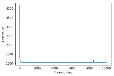
plt.plot(iaf_loss)
plt.xlabel('Training step')
_ = plt.ylabel('Loss value')
IAF surrogate posterior ELBO: -1065.3663330078125
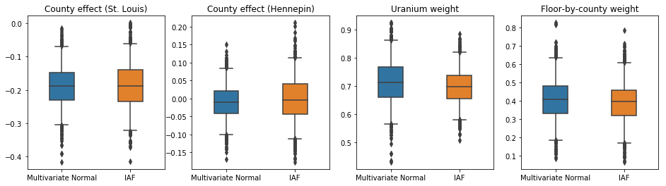
IAF 代理后验的可信区间与受约束的多元正态的可信区间相似。
results['IAF'] = pack_samples(iaf_samples)
plot_boxplot(results)
基线:平均场代理后验
VI 代理后验通常被假定为平均场(独立)正态分布,具有可训练的均值和方差,它们通过双射变换受限于先验的支持。除了两个更具表现力的代理后验之外,我们还使用与多元正态代理后验相同的通用公式定义了一个平均场代理后验。
# A block-diagonal linear operator, in which each block is a diagonal operator,
# transforms the standard Normal base distribution to produce a mean-field
# surrogate posterior.
operators = (tf.linalg.LinearOperatorDiag,
             tf.linalg.LinearOperatorDiag,
             tf.linalg.LinearOperatorDiag)
block_diag_linop = (
    tfp.experimental.vi.util.build_trainable_linear_operator_block(
        operators, flat_event_size))
mean_field_scale = tfb.ScaleMatvecLinearOperatorBlock(block_diag_linop)

mean_field_loc = tfb.JointMap(
    tf.nest.map_structure(
        lambda s: tfb.Shift(
            tf.Variable(tf.random.uniform(
                (s,), minval=-2., maxval=2., dtype=tf.float32))),
        flat_event_size))

mean_field_surrogate_posterior = tfd.TransformedDistribution(
    base_standard_dist,
    bijector = tfb.Chain(  # Note that the chained bijectors are applied in reverse order
        [
         event_space_bijector,  # constrain the surrogate to the support of the prior
         unflatten_bijector,  # pack the reshaped components into the `event_shape` structure of the posterior
         reshape_bijector, # reshape the vector-valued components to match the shapes of the posterior components
         mean_field_loc,   # allow for nonzero mean
         mean_field_scale  # apply the block matrix transformation to the standard Normal distribution
         ]))

optimizer=tf.optimizers.Adam(learning_rate=1e-2)
mean_field_loss = tfp.vi.fit_surrogate_posterior(
    target_model.unnormalized_log_prob,
    mean_field_surrogate_posterior,
    optimizer=optimizer,
    num_steps=10**4,
    sample_size=16,
    jit_compile=True)

mean_field_samples = mean_field_surrogate_posterior.sample(1000)
mean_field_final_elbo = tf.reduce_mean(
    target_model.unnormalized_log_prob(*mean_field_samples)
    - mean_field_surrogate_posterior.log_prob(mean_field_samples))
print('Mean-field surrogate posterior ELBO: {}'.format(mean_field_final_elbo))

plt.plot(mean_field_loss)
plt.xlabel('Training step')
_ = plt.ylabel('Loss value')
Mean-field surrogate posterior ELBO: -1065.7652587890625
在这种情况下,平均场代理后验给出了与更具表现力的代理后验相似的结果,表明这种更简单的模型可能足以完成推断任务。
results['Mean Field'] = pack_samples(mean_field_samples)
plot_boxplot(results)
真实:哈密顿蒙特卡罗 (HMC)
我们使用 HMC 从真实的后验中生成“真实”样本,用于与代理后验的结果进行比较。
num_chains = 8
num_leapfrog_steps = 3
step_size = 0.4
num_steps=20000

flat_event_shape = tf.nest.flatten(target_model.event_shape)
enum_components = list(range(len(flat_event_shape)))
bijector = tfb.Restructure(
    enum_components,
    tf.nest.pack_sequence_as(target_model.event_shape, enum_components))(
        target_model.experimental_default_event_space_bijector())

current_state = bijector(
    tf.nest.map_structure(
        lambda e: tf.zeros([num_chains] + list(e), dtype=tf.float32),
    target_model.event_shape))

hmc = tfp.mcmc.HamiltonianMonteCarlo(
    target_log_prob_fn=target_model.unnormalized_log_prob,
    num_leapfrog_steps=num_leapfrog_steps,
    step_size=[tf.fill(s.shape, step_size) for s in current_state])

hmc = tfp.mcmc.TransformedTransitionKernel(
    hmc, bijector)
hmc = tfp.mcmc.DualAveragingStepSizeAdaptation(
    hmc,
    num_adaptation_steps=int(num_steps // 2 * 0.8),
    target_accept_prob=0.9)

chain, is_accepted = tf.function(
    lambda current_state: tfp.mcmc.sample_chain(
        current_state=current_state,
        kernel=hmc,
        num_results=num_steps // 2,
        num_burnin_steps=num_steps // 2,
        trace_fn=lambda _, pkr:
        (pkr.inner_results.inner_results.is_accepted),
        ),
    autograph=False,
    jit_compile=True)(current_state)

accept_rate = tf.reduce_mean(tf.cast(is_accepted, tf.float32))
ess = tf.nest.map_structure(
    lambda c: tfp.mcmc.effective_sample_size(
        c,
        cross_chain_dims=1,
        filter_beyond_positive_pairs=True),
    chain)

r_hat = tf.nest.map_structure(tfp.mcmc.potential_scale_reduction, chain)
hmc_samples = pack_samples(
    tf.nest.pack_sequence_as(target_model.event_shape, chain))
print('Acceptance rate is {}'.format(accept_rate))
Acceptance rate is 0.9008625149726868
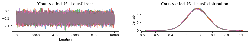
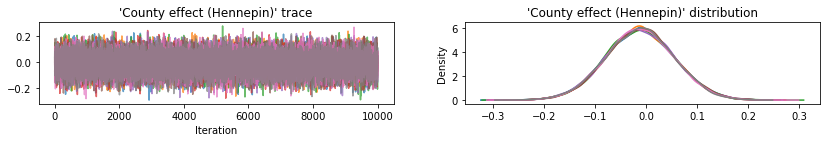
绘制样本轨迹以检查 HMC 结果的完整性。
def plot_traces(var_name, samples):
  fig, axes = plt.subplots(1, 2, figsize=(14, 1.5), sharex='col', sharey='col')
  for chain in range(num_chains):
    s = samples.numpy()[:, chain]
    axes[0].plot(s, alpha=0.7)
    sns.kdeplot(s, ax=axes[1], shade=False)
    axes[0].title.set_text("'{}' trace".format(var_name))
    axes[1].title.set_text("'{}' distribution".format(var_name))
    axes[0].set_xlabel('Iteration')

warnings.filterwarnings('ignore')
for var, var_samples in hmc_samples.items():
  plot_traces(var, var_samples)
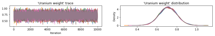
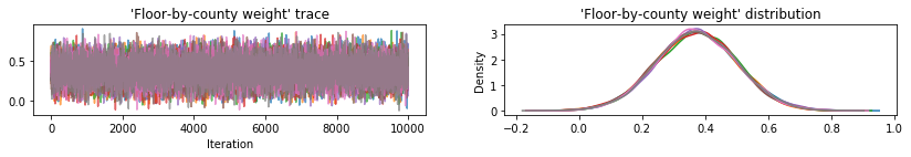
所有三个代理后验都产生了在视觉上与 HMC 样本相似的可信区间,尽管有时由于 ELBO 损失的影响而分散不足,但这在 VI 中很常见。
results['HMC'] = hmc_samples
plot_boxplot(results)
附加结果
Plotting functions
plt.rcParams.update({'axes.titlesize': 'medium', 'xtick.labelsize': 'medium'})
def plot_loss_and_elbo():
  fig, axes = plt.subplots(1, 2, figsize=(12, 4))

  axes[0].scatter([0, 1, 2],
                  [mvn_final_elbo.numpy(),
                  iaf_final_elbo.numpy(),
                  mean_field_final_elbo.numpy()])
  axes[0].set_xticks(ticks=[0, 1, 2])
  axes[0].set_xticklabels(labels=[
    'Multivariate Normal', 'IAF', 'Mean Field'])
  axes[0].title.set_text('Evidence Lower Bound (ELBO)')

  axes[1].plot(mvn_loss, label='Multivariate Normal')
  axes[1].plot(iaf_loss, label='IAF')
  axes[1].plot(mean_field_loss, label='Mean Field')
  axes[1].set_ylim([1000, 4000])
  axes[1].set_xlabel('Training step')
  axes[1].set_ylabel('Loss (negative ELBO)')
  axes[1].title.set_text('Loss')
  plt.legend()
  plt.show()

plt.rcParams.update({'axes.titlesize': 'medium', 'xtick.labelsize': 'small'})
def plot_kdes(num_chains=8):
  fig, axes = plt.subplots(2, 2, figsize=(12, 8))
  k = list(results.values())[0].keys()
  plot_results = {
      v: {p: results[p][v] for p in results} for v in k}
  for i, (var, var_results) in enumerate(plot_results.items()):
    ax = axes[i % 2, i // 2]
    for posterior, posterior_results in var_results.items():
      if posterior == 'HMC':
        label = posterior
        for chain in range(num_chains):
          sns.kdeplot(
              posterior_results[:, chain],
              ax=ax, shade=False, color='k', linestyle=':', label=label)
          label=None
      else:
        sns.kdeplot(
            posterior_results, ax=ax, shade=False, label=posterior)
        ax.title.set_text('{}'.format(var))
    ax.legend()
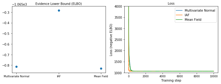
证据下界 (ELBO)
IAF 是迄今为止最大和最灵活的代理后验,收敛于最高的证据下界 (ELBO)。
plot_loss_and_elbo()
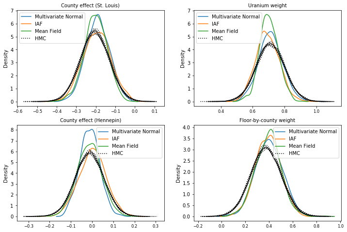
后验样本
来自每个代理后验的样本与 HMC 真实样本进行比较(箱形图中显示的不同的样本可视化)。
plot_kdes()
结论
在本 Colab 中,我们使用联合分布和多部分双射函数构建了 VI 代理后验,并对它们进行拟合以估计氡数据集回归模型中权重的可信区间。对于这个简单的模型,更具表现力的代理后验与平均场代理后验的表现相似。然而,我们展示的工具可用于构建各种灵活的适用于更复杂模型的代理后验。