
| | |  Wyświetl źródło na GitHub Wyświetl źródło na GitHub |
Ten notebook trenuje sekwencję modelu sekwencji (seq2seq) dla hiszpańskich tłumaczeniu angielskim w oparciu o skuteczne podejścia opartego na baczność Neural tłumaczenia maszynowego . To jest zaawansowany przykład, który zakłada pewną wiedzę na temat:
- Sekwencja do modeli sekwencji
- Podstawy TensorFlow pod warstwą keras:
- Bezpośrednia praca z tensorami
- Pisanie zwyczaj
keras.Models ikeras.layers
Choć architektura jest nieco nieaktualne nadal jest to bardzo użyteczne do pracy poprzez projekt, aby uzyskać głębsze zrozumienie mechanizmów uwagi (przed przejściem do Transformers ).
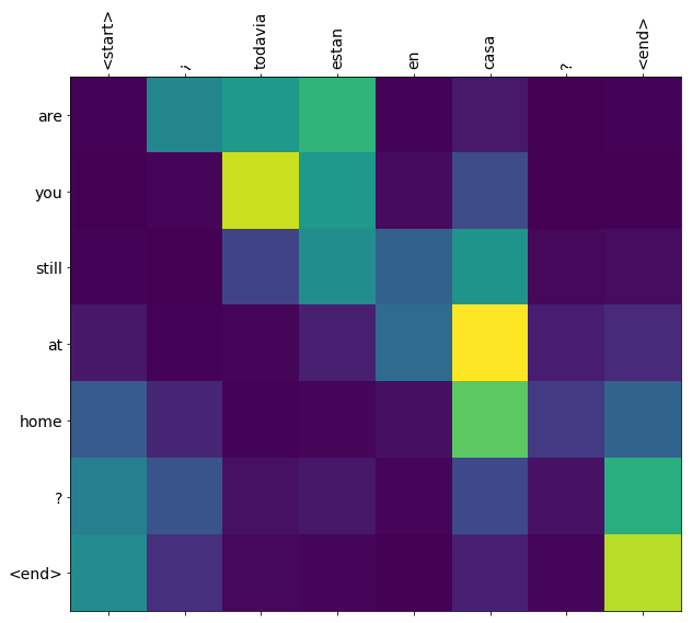
Po treningu w tym modelu notebooka, będzie można do wejścia zdaniu hiszpańskiej, jak i powrót angielskie tłumaczenie „¿todavia estan en casa?”: „Czy wciąż jesteś w domu”
Otrzymany model jest eksportowane jako tf.saved_model , dzięki czemu można go stosować w innych środowiskach TensorFlow.
Jakość tłumaczenia jest rozsądna jak na przykład zabawkowy, ale wygenerowany wątek uwagi jest być może bardziej interesujący. Pokazuje to, na które części zdania wejściowego zwraca uwagę model podczas tłumaczenia:
Ustawiać
pip install tensorflow_text
import numpy as np

import typing
from typing import Any, Tuple

import tensorflow as tf

import tensorflow_text as tf_text

import matplotlib.pyplot as plt
import matplotlib.ticker as ticker
Ten samouczek buduje kilka warstw od podstaw, użyj tej zmiennej, jeśli chcesz przełączać się między implementacją niestandardową i wbudowaną.
use_builtins = True
Ten samouczek korzysta z wielu niskopoziomowych interfejsów API, w których łatwo jest pomylić kształty. Ta klasa służy do sprawdzania kształtów w tym samouczku.
Kontroler kształtu
class ShapeChecker():
  def __init__(self):
    # Keep a cache of every axis-name seen
    self.shapes = {}

  def __call__(self, tensor, names, broadcast=False):
    if not tf.executing_eagerly():
      return

    if isinstance(names, str):
      names = (names,)

    shape = tf.shape(tensor)
    rank = tf.rank(tensor)

    if rank != len(names):
      raise ValueError(f'Rank mismatch:\n'
                       f'    found {rank}: {shape.numpy()}\n'
                       f'    expected {len(names)}: {names}\n')

    for i, name in enumerate(names):
      if isinstance(name, int):
        old_dim = name
      else:
        old_dim = self.shapes.get(name, None)
      new_dim = shape[i]

      if (broadcast and new_dim == 1):
        continue

      if old_dim is None:
        # If the axis name is new, add its length to the cache.
        self.shapes[name] = new_dim
        continue

      if new_dim != old_dim:
        raise ValueError(f"Shape mismatch for dimension: '{name}'\n"
                         f"    found: {new_dim}\n"
                         f"    expected: {old_dim}\n")
Dane
Użyjemy zestawu danych dostarczonych przez język http://www.manythings.org/anki/ Ten zestaw danych zawiera pary tłumaczy w formacie:
May I borrow this book? ¿Puedo tomar prestado este libro?
Dostępne są różne języki, ale my użyjemy zestawu danych angielsko-hiszpański.
Pobierz i przygotuj zbiór danych
Dla wygody umieściliśmy kopię tego zbioru danych w Google Cloud, ale możesz też pobrać własną kopię. Po pobraniu zestawu danych, oto kroki, które podejmiemy, aby przygotować dane:
- Dodaj początek i koniec żeton do każdego zdania.
- Wyczyść zdania, usuwając znaki specjalne.
- Utwórz indeks słów i indeks słów odwrotnych (odwzorowanie słowników ze słowa → id i id → słowo).
- Uzupełnij każde zdanie do maksymalnej długości.
# Download the file
import pathlib

path_to_zip = tf.keras.utils.get_file(
    'spa-eng.zip', origin='http://storage.googleapis.com/download.tensorflow.org/data/spa-eng.zip',
    extract=True)

path_to_file = pathlib.Path(path_to_zip).parent/'spa-eng/spa.txt'
Downloading data from http://storage.googleapis.com/download.tensorflow.org/data/spa-eng.zip
2646016/2638744 [==============================] - 0s 0us/step
2654208/2638744 [==============================] - 0s 0us/step
def load_data(path):
  text = path.read_text(encoding='utf-8')

  lines = text.splitlines()
  pairs = [line.split('\t') for line in lines]

  inp = [inp for targ, inp in pairs]
  targ = [targ for targ, inp in pairs]

  return targ, inp
targ, inp = load_data(path_to_file)
print(inp[-1])
Si quieres sonar como un hablante nativo, debes estar dispuesto a practicar diciendo la misma frase una y otra vez de la misma manera en que un músico de banjo practica el mismo fraseo una y otra vez hasta que lo puedan tocar correctamente y en el tiempo esperado.
print(targ[-1])
If you want to sound like a native speaker, you must be willing to practice saying the same sentence over and over in the same way that banjo players practice the same phrase over and over until they can play it correctly and at the desired tempo.
Utwórz zbiór danych tf.data
Z tych tablic ciągów można utworzyć tf.data.Dataset że tasuje je i partie skutecznie ciągów:
BUFFER_SIZE = len(inp)
BATCH_SIZE = 64

dataset = tf.data.Dataset.from_tensor_slices((inp, targ)).shuffle(BUFFER_SIZE)
dataset = dataset.batch(BATCH_SIZE)
for example_input_batch, example_target_batch in dataset.take(1):
  print(example_input_batch[:5])
  print()
  print(example_target_batch[:5])
  break
tf.Tensor(
[b'No s\xc3\xa9 lo que quiero.' b'\xc2\xbfDeber\xc3\xada repetirlo?'
 b'Tard\xc3\xa9 m\xc3\xa1s de 2 horas en traducir unas p\xc3\xa1ginas en ingl\xc3\xa9s.'
 b'A Tom comenz\xc3\xb3 a temerle a Mary.' b'Mi pasatiempo es la lectura.'], shape=(5,), dtype=string)

tf.Tensor(
[b"I don't know what I want." b'Should I repeat it?'
 b'It took me more than two hours to translate a few pages of English.'
 b'Tom became afraid of Mary.' b'My hobby is reading.'], shape=(5,), dtype=string)
Wstępne przetwarzanie tekstu
Jednym z celów tego poradnika jest zbudowanie modelu, które mogą być eksportowane jako tf.saved_model . Aby wywożony modelu przydatny powinien upłynąć tf.string wejść i powrócić tf.string wyjść: Wszystkie przetwarzanie tekstu dzieje się wewnątrz modelu.
Normalizacja
Model zajmuje się tekstem wielojęzycznym z ograniczonym słownictwem. Dlatego ważne będzie ujednolicenie tekstu wejściowego.
Pierwszym krokiem jest normalizacja Unicode w celu podzielenia znaków akcentowanych i zastąpienia znaków zgodności ich odpowiednikami ASCII.
tensorflow_text Pakiet zawiera obsługę Unicode normalizować:
example_text = tf.constant('¿Todavía está en casa?')

print(example_text.numpy())
print(tf_text.normalize_utf8(example_text, 'NFKD').numpy())
b'\xc2\xbfTodav\xc3\xada est\xc3\xa1 en casa?'
b'\xc2\xbfTodavi\xcc\x81a esta\xcc\x81 en casa?'
Normalizacja Unicode będzie pierwszym krokiem w funkcji standaryzacji tekstu:
def tf_lower_and_split_punct(text):
  # Split accecented characters.
  text = tf_text.normalize_utf8(text, 'NFKD')
  text = tf.strings.lower(text)
  # Keep space, a to z, and select punctuation.
  text = tf.strings.regex_replace(text, '[^ a-z.?!,¿]', '')
  # Add spaces around punctuation.
  text = tf.strings.regex_replace(text, '[.?!,¿]', r' \0 ')
  # Strip whitespace.
  text = tf.strings.strip(text)

  text = tf.strings.join(['[START]', text, '[END]'], separator=' ')
  return text
print(example_text.numpy().decode())
print(tf_lower_and_split_punct(example_text).numpy().decode())
¿Todavía está en casa?
[START] ¿ todavia esta en casa ? [END]
Wektoryzacja tekstu
Funkcja normalizacji zostanie owinięte w tf.keras.layers.TextVectorization warstwy, która będzie obsługiwać ekstrakcji słownikowy i konwersji tekstu wejściowego do sekwencji słów.
max_vocab_size = 5000

input_text_processor = tf.keras.layers.TextVectorization(
    standardize=tf_lower_and_split_punct,
    max_tokens=max_vocab_size)
TextVectorization warstwy i wiele innych warstw przerób mieć adapt sposobu. Metoda ta odczytuje jedną epokę danych szkolenia i działa trochę jak Model.fix . Ten adapt sposób inicjuje warstwę opartą na danych. Tutaj określa słownictwo:
input_text_processor.adapt(inp)

# Here are the first 10 words from the vocabulary:
input_text_processor.get_vocabulary()[:10]
['', '[UNK]', '[START]', '[END]', '.', 'que', 'de', 'el', 'a', 'no']
To hiszpański TextVectorization warstwa, teraz budować i .adapt() Anglicy jeden:
output_text_processor = tf.keras.layers.TextVectorization(
    standardize=tf_lower_and_split_punct,
    max_tokens=max_vocab_size)

output_text_processor.adapt(targ)
output_text_processor.get_vocabulary()[:10]
['', '[UNK]', '[START]', '[END]', '.', 'the', 'i', 'to', 'you', 'tom']
Teraz te warstwy mogą konwertować partię ciągów na partię identyfikatorów tokenów:
example_tokens = input_text_processor(example_input_batch)
example_tokens[:3, :10]
<tf.Tensor: shape=(3, 10), dtype=int64, numpy=
array([[   2,    9,   17,   22,    5,   48,    4,    3,    0,    0],
       [   2,   13,  177,    1,   12,    3,    0,    0,    0,    0],
       [   2,  120,   35,    6,  290,   14, 2134,  506, 2637,   14]])>
get_vocabulary metoda może być użyty do konwersji identyfikatorów tokenów z powrotem do tekstu:
input_vocab = np.array(input_text_processor.get_vocabulary())
tokens = input_vocab[example_tokens[0].numpy()]
' '.join(tokens)
'[START] no se lo que quiero . [END] '
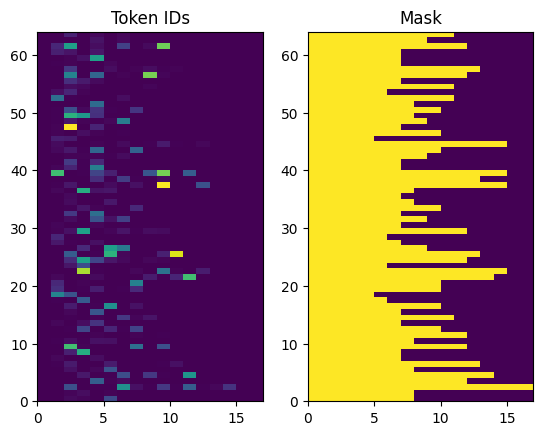
Zwrócone identyfikatory tokenów są uzupełniane zerami. Można to łatwo zamienić w maskę:
plt.subplot(1, 2, 1)
plt.pcolormesh(example_tokens)
plt.title('Token IDs')

plt.subplot(1, 2, 2)
plt.pcolormesh(example_tokens != 0)
plt.title('Mask')
Text(0.5, 1.0, 'Mask')
Model enkodera/dekodera
Poniższy diagram przedstawia przegląd modelu. W każdym kroku czasowym dane wyjściowe dekodera są łączone z ważoną sumą zakodowanych danych wejściowych, aby przewidzieć następne słowo. Schemat i wzory są z papieru Luong za .

Zanim się do tego zabierzesz zdefiniuj kilka stałych dla modelu:
embedding_dim = 256
units = 1024
Koder
Zacznij od zbudowania enkodera, niebieskiej części powyższego diagramu.
Koder:
- Przyjmuje listę identyfikatorów tokenów (od
input_text_processor). - Patrzy na osadzanie wektora dla każdego tokena (Korzystanie z
layers.Embedding). - Przetwarza zanurzeń do nowej sekwencji (przy użyciu
layers.GRU). - Zwroty:
- Przetworzona sekwencja. Zostanie to przekazane do głowy uwagi.
- Stan wewnętrzny. Będzie to użyte do inicjalizacji dekodera
class Encoder(tf.keras.layers.Layer):
  def __init__(self, input_vocab_size, embedding_dim, enc_units):
    super(Encoder, self).__init__()
    self.enc_units = enc_units
    self.input_vocab_size = input_vocab_size

    # The embedding layer converts tokens to vectors
    self.embedding = tf.keras.layers.Embedding(self.input_vocab_size,
                                               embedding_dim)

    # The GRU RNN layer processes those vectors sequentially.
    self.gru = tf.keras.layers.GRU(self.enc_units,
                                   # Return the sequence and state
                                   return_sequences=True,
                                   return_state=True,
                                   recurrent_initializer='glorot_uniform')

  def call(self, tokens, state=None):
    shape_checker = ShapeChecker()
    shape_checker(tokens, ('batch', 's'))

    # 2. The embedding layer looks up the embedding for each token.
    vectors = self.embedding(tokens)
    shape_checker(vectors, ('batch', 's', 'embed_dim'))

    # 3. The GRU processes the embedding sequence.
    #    output shape: (batch, s, enc_units)
    #    state shape: (batch, enc_units)
    output, state = self.gru(vectors, initial_state=state)
    shape_checker(output, ('batch', 's', 'enc_units'))
    shape_checker(state, ('batch', 'enc_units'))

    # 4. Returns the new sequence and its state.
    return output, state
Oto, jak do tej pory pasuje do siebie:
# Convert the input text to tokens.
example_tokens = input_text_processor(example_input_batch)

# Encode the input sequence.
encoder = Encoder(input_text_processor.vocabulary_size(),
                  embedding_dim, units)
example_enc_output, example_enc_state = encoder(example_tokens)

print(f'Input batch, shape (batch): {example_input_batch.shape}')
print(f'Input batch tokens, shape (batch, s): {example_tokens.shape}')
print(f'Encoder output, shape (batch, s, units): {example_enc_output.shape}')
print(f'Encoder state, shape (batch, units): {example_enc_state.shape}')
Input batch, shape (batch): (64,)
Input batch tokens, shape (batch, s): (64, 14)
Encoder output, shape (batch, s, units): (64, 14, 1024)
Encoder state, shape (batch, units): (64, 1024)
Koder zwraca swój stan wewnętrzny, dzięki czemu jego stan można wykorzystać do zainicjowania dekodera.
Często zdarza się również, że RNN zwraca swój stan, aby mógł przetwarzać sekwencję w wielu wywołaniach. Zobaczysz więcej tego budowania dekodera.
Głowa uwagi
Dekoder zwraca uwagę, aby selektywnie skupiać się na częściach sekwencji wejściowej. Uwaga pobiera sekwencję wektorów jako dane wejściowe dla każdego przykładu i zwraca wektor „uwagi” dla każdego przykładu. Ta warstwa uwagi jest podobny do layers.GlobalAveragePoling1D ale warstwa uwagę wykonuje średniej ważonej.
Zobaczmy, jak to działa:


Gdzie:
- \(s\) jest indeksem enkodera.
- \(t\) jest indeksem dekoder.
- \(\alpha_{ts}\) jest ciężary uwagę.
- \(h_s\) jest sekwencją wyjścia kodera jest uczęszczanych ( „klucz” uwagi i „wartość” w terminologii transformatora).
- \(h_t\) jest stan dekoder udział sekwencji (uwaga „zapytania” w terminologii transformatora).
- \(c_t\) jest Otrzymany wektor kontekst.
- \(a_t\) jest Wyjście końcowe łączenie „kontekst” i „hasła”.
Równania:
- Oblicza ciężarów uwaga, \(\alpha_{ts}\)jako Softmax całej sekwencji wyjścia enkodera.
- Oblicza wektor kontekstu jako ważoną sumę danych wyjściowych kodera.
Ostatni jest \(score\) funkcja. Jego zadaniem jest obliczenie skalarnego wyniku logitowego dla każdej pary klucz-zapytanie. Istnieją dwa popularne podejścia:

Ten tutorial używa dodatków uwagę Bahdanau użytkownika . TensorFlow zawiera implementacje zarówno jako layers.Attention i layers.AdditiveAttention . Klasa poniżej obsługuje macierze wagowe w parze layers.Dense warstw i wzywa realizację wbudowanego.
class BahdanauAttention(tf.keras.layers.Layer):
  def __init__(self, units):
    super().__init__()
    # For Eqn. (4), the  Bahdanau attention
    self.W1 = tf.keras.layers.Dense(units, use_bias=False)
    self.W2 = tf.keras.layers.Dense(units, use_bias=False)

    self.attention = tf.keras.layers.AdditiveAttention()

  def call(self, query, value, mask):
    shape_checker = ShapeChecker()
    shape_checker(query, ('batch', 't', 'query_units'))
    shape_checker(value, ('batch', 's', 'value_units'))
    shape_checker(mask, ('batch', 's'))

    # From Eqn. (4), `W1@ht`.
    w1_query = self.W1(query)
    shape_checker(w1_query, ('batch', 't', 'attn_units'))

    # From Eqn. (4), `W2@hs`.
    w2_key = self.W2(value)
    shape_checker(w2_key, ('batch', 's', 'attn_units'))

    query_mask = tf.ones(tf.shape(query)[:-1], dtype=bool)
    value_mask = mask

    context_vector, attention_weights = self.attention(
        inputs = [w1_query, value, w2_key],
        mask=[query_mask, value_mask],
        return_attention_scores = True,
    )
    shape_checker(context_vector, ('batch', 't', 'value_units'))
    shape_checker(attention_weights, ('batch', 't', 's'))

    return context_vector, attention_weights
Przetestuj warstwę uwagi
Tworzenie BahdanauAttention warstwy:
attention_layer = BahdanauAttention(units)
Ta warstwa wymaga 3 wejść:
-
query: To będzie generowana przez dekoder, później. -
value: To będzie wyjście kodera. -
mask: Aby wykluczyć wyściółkę,example_tokens != 0
(example_tokens != 0).shape
TensorShape([64, 14])
Zwektoryzowana implementacja warstwy uwagi umożliwia przekazanie serii sekwencji wektorów zapytań oraz serii sekwencji wektorów wartości. Wynik to:
- Partia sekwencji wektorów wynikowych wielkości zapytań.
- Partia uwaga mapy o wielkości
(query_length, value_length).
# Later, the decoder will generate this attention query
example_attention_query = tf.random.normal(shape=[len(example_tokens), 2, 10])

# Attend to the encoded tokens

context_vector, attention_weights = attention_layer(
    query=example_attention_query,
    value=example_enc_output,
    mask=(example_tokens != 0))

print(f'Attention result shape: (batch_size, query_seq_length, units):           {context_vector.shape}')
print(f'Attention weights shape: (batch_size, query_seq_length, value_seq_length): {attention_weights.shape}')
Attention result shape: (batch_size, query_seq_length, units):           (64, 2, 1024)
Attention weights shape: (batch_size, query_seq_length, value_seq_length): (64, 2, 14)
Ciężary uwagę należy zsumować do 1.0 dla każdej sekwencji.
Oto uwaga wagi całej sekwencji w t=0 :
plt.subplot(1, 2, 1)
plt.pcolormesh(attention_weights[:, 0, :])
plt.title('Attention weights')

plt.subplot(1, 2, 2)
plt.pcolormesh(example_tokens != 0)
plt.title('Mask')
Text(0.5, 1.0, 'Mask')

Ze względu na małą losowej inicjalizacji wagi uwaga są blisko 1/(sequence_length) . Jeśli powiększyć wag dla pojedynczej sekwencji, można zobaczyć, że jest jakaś mała zmienność, że model może się nauczyć, aby rozwinąć i wykorzystać.
attention_weights.shape
TensorShape([64, 2, 14])
attention_slice = attention_weights[0, 0].numpy()
attention_slice = attention_slice[attention_slice != 0]
plt.suptitle('Attention weights for one sequence')

plt.figure(figsize=(12, 6))
a1 = plt.subplot(1, 2, 1)
plt.bar(range(len(attention_slice)), attention_slice)
# freeze the xlim
plt.xlim(plt.xlim())
plt.xlabel('Attention weights')

a2 = plt.subplot(1, 2, 2)
plt.bar(range(len(attention_slice)), attention_slice)
plt.xlabel('Attention weights, zoomed')

# zoom in
top = max(a1.get_ylim())
zoom = 0.85*top
a2.set_ylim([0.90*top, top])
a1.plot(a1.get_xlim(), [zoom, zoom], color='k')
[<matplotlib.lines.Line2D at 0x7fb42c5b1090>]
<Figure size 432x288 with 0 Axes>

Dekoder
Zadaniem dekodera jest generowanie predykcji dla następnego tokena wyjściowego.
- Dekoder odbiera pełne dane wyjściowe kodera.
- Wykorzystuje RNN do śledzenia tego, co do tej pory wygenerowało.
- Wykorzystuje swoje wyjście RNN jako zapytanie zwracające uwagę na wyjście kodera, tworząc wektor kontekstu.
- Łączy dane wyjściowe RNN i wektor kontekstu przy użyciu równania 3 (poniżej) w celu wygenerowania „wektora uwagi”.
- Generuje prognozy logitowe dla następnego tokena na podstawie „wektora uwagi”.

Oto Decoder klasy i jej inicjator. Inicjator tworzy wszystkie niezbędne warstwy.
class Decoder(tf.keras.layers.Layer):
  def __init__(self, output_vocab_size, embedding_dim, dec_units):
    super(Decoder, self).__init__()
    self.dec_units = dec_units
    self.output_vocab_size = output_vocab_size
    self.embedding_dim = embedding_dim

    # For Step 1. The embedding layer convets token IDs to vectors
    self.embedding = tf.keras.layers.Embedding(self.output_vocab_size,
                                               embedding_dim)

    # For Step 2. The RNN keeps track of what's been generated so far.
    self.gru = tf.keras.layers.GRU(self.dec_units,
                                   return_sequences=True,
                                   return_state=True,
                                   recurrent_initializer='glorot_uniform')

    # For step 3. The RNN output will be the query for the attention layer.
    self.attention = BahdanauAttention(self.dec_units)

    # For step 4. Eqn. (3): converting `ct` to `at`
    self.Wc = tf.keras.layers.Dense(dec_units, activation=tf.math.tanh,
                                    use_bias=False)

    # For step 5. This fully connected layer produces the logits for each
    # output token.
    self.fc = tf.keras.layers.Dense(self.output_vocab_size)
call metody dla tej warstwy przyjmuje i zwraca wiele tensorów. Zorganizuj je w proste klasy kontenerów:
class DecoderInput(typing.NamedTuple):
  new_tokens: Any
  enc_output: Any
  mask: Any

class DecoderOutput(typing.NamedTuple):
  logits: Any
  attention_weights: Any
Tutaj jest realizacja call metodą:
def call(self,
         inputs: DecoderInput,
         state=None) -> Tuple[DecoderOutput, tf.Tensor]:
  shape_checker = ShapeChecker()
  shape_checker(inputs.new_tokens, ('batch', 't'))
  shape_checker(inputs.enc_output, ('batch', 's', 'enc_units'))
  shape_checker(inputs.mask, ('batch', 's'))

  if state is not None:
    shape_checker(state, ('batch', 'dec_units'))

  # Step 1. Lookup the embeddings
  vectors = self.embedding(inputs.new_tokens)
  shape_checker(vectors, ('batch', 't', 'embedding_dim'))

  # Step 2. Process one step with the RNN
  rnn_output, state = self.gru(vectors, initial_state=state)

  shape_checker(rnn_output, ('batch', 't', 'dec_units'))
  shape_checker(state, ('batch', 'dec_units'))

  # Step 3. Use the RNN output as the query for the attention over the
  # encoder output.
  context_vector, attention_weights = self.attention(
      query=rnn_output, value=inputs.enc_output, mask=inputs.mask)
  shape_checker(context_vector, ('batch', 't', 'dec_units'))
  shape_checker(attention_weights, ('batch', 't', 's'))

  # Step 4. Eqn. (3): Join the context_vector and rnn_output
  #     [ct; ht] shape: (batch t, value_units + query_units)
  context_and_rnn_output = tf.concat([context_vector, rnn_output], axis=-1)

  # Step 4. Eqn. (3): `at = tanh(Wc@[ct; ht])`
  attention_vector = self.Wc(context_and_rnn_output)
  shape_checker(attention_vector, ('batch', 't', 'dec_units'))

  # Step 5. Generate logit predictions:
  logits = self.fc(attention_vector)
  shape_checker(logits, ('batch', 't', 'output_vocab_size'))

  return DecoderOutput(logits, attention_weights), state
Decoder.call = call
Koder przetwarza pełną sekwencję wejściową z pojedynczym wywołaniu jej RNN. Ta implementacja dekodera można zrobić również dla efektywnego treningu. Ale ten samouczek uruchomi dekoder w pętli z kilku powodów:
- Elastyczność: Pisanie pętli daje bezpośrednią kontrolę nad procedurą treningu.
- Klarowność: To jest możliwe do zrobienia maskujące sztuczki i korzystać
layers.RNNlubtfa.seq2seqAPI zapakować to wszystko w jednym połączeniu. Ale zapisanie tego jako pętli może być jaśniejsze.- Pętla darmowe szkolenie wykazano w generacji Tekst tutiorial.
Teraz spróbuj użyć tego dekodera.
decoder = Decoder(output_text_processor.vocabulary_size(),
                  embedding_dim, units)
Dekoder przyjmuje 4 wejścia.
-
new_tokens- ostatni żeton generowane. Zainicjować dekoder z"[START]"tokenu. -
enc_output- Generowane przezEncoder. -
mask- tensor logiczny wskazujący gdzietokens != 0 -
state- Dotychczasowystatewyjściowy z dekodera (stan wewnętrznego dekodera RNN). PrzechodząNonezero-go zainicjować. Oryginalny dokument inicjuje go z końcowego stanu RNN kodera.
# Convert the target sequence, and collect the "[START]" tokens
example_output_tokens = output_text_processor(example_target_batch)

start_index = output_text_processor.get_vocabulary().index('[START]')
first_token = tf.constant([[start_index]] * example_output_tokens.shape[0])
# Run the decoder
dec_result, dec_state = decoder(
    inputs = DecoderInput(new_tokens=first_token,
                          enc_output=example_enc_output,
                          mask=(example_tokens != 0)),
    state = example_enc_state
)

print(f'logits shape: (batch_size, t, output_vocab_size) {dec_result.logits.shape}')
print(f'state shape: (batch_size, dec_units) {dec_state.shape}')
logits shape: (batch_size, t, output_vocab_size) (64, 1, 5000)
state shape: (batch_size, dec_units) (64, 1024)
Wypróbuj token zgodnie z logami:
sampled_token = tf.random.categorical(dec_result.logits[:, 0, :], num_samples=1)
Dekoduj token jako pierwsze słowo wyjścia:
vocab = np.array(output_text_processor.get_vocabulary())
first_word = vocab[sampled_token.numpy()]
first_word[:5]
array([['already'],
       ['plants'],
       ['pretended'],
       ['convince'],
       ['square']], dtype='<U16')
Teraz użyj dekodera, aby wygenerować drugi zestaw logitów.
- Przekazać tę samą
enc_outputimaskte nie uległy zmianie. - Przejść Próbkowany żeton w
new_tokens. - Przepuścić
decoder_statedekoder zwrócony po raz ostatni, więc RNN nadal z pamięci, gdzie zostało przerwane po raz ostatni.
dec_result, dec_state = decoder(
    DecoderInput(sampled_token,
                 example_enc_output,
                 mask=(example_tokens != 0)),
    state=dec_state)
sampled_token = tf.random.categorical(dec_result.logits[:, 0, :], num_samples=1)
first_word = vocab[sampled_token.numpy()]
first_word[:5]
array([['nap'],
       ['mean'],
       ['worker'],
       ['passage'],
       ['baked']], dtype='<U16')
Trening
Teraz, gdy masz już wszystkie składniki modelu, nadszedł czas, aby rozpocząć trenowanie modelu. Będziesz potrzebował:
- Funkcja straty i optymalizator do przeprowadzenia optymalizacji.
- Funkcja kroku szkolenia definiująca sposób aktualizowania modelu dla każdej partii wejściowej/docelowej.
- Pętla treningowa do prowadzenia treningu i zapisywania punktów kontrolnych.
Zdefiniuj funkcję straty
class MaskedLoss(tf.keras.losses.Loss):
  def __init__(self):
    self.name = 'masked_loss'
    self.loss = tf.keras.losses.SparseCategoricalCrossentropy(
        from_logits=True, reduction='none')

  def __call__(self, y_true, y_pred):
    shape_checker = ShapeChecker()
    shape_checker(y_true, ('batch', 't'))
    shape_checker(y_pred, ('batch', 't', 'logits'))

    # Calculate the loss for each item in the batch.
    loss = self.loss(y_true, y_pred)
    shape_checker(loss, ('batch', 't'))

    # Mask off the losses on padding.
    mask = tf.cast(y_true != 0, tf.float32)
    shape_checker(mask, ('batch', 't'))
    loss *= mask

    # Return the total.
    return tf.reduce_sum(loss)
Zrealizuj etap szkolenia
Start z klasy modelu, proces szkolenia będą realizowane jako train_step metody na tym modelu. Patrz Dostosowywanie pasuje do szczegółów.
Tutaj train_step metoda jest owinięcie wokół _train_step realizacji, która będzie później. Owijka ta zawiera przełącznik do włączania i wyłączania tf.function kompilacji, aby ułatwić debugowanie.
class TrainTranslator(tf.keras.Model):
  def __init__(self, embedding_dim, units,
               input_text_processor,
               output_text_processor,
               use_tf_function=True):
    super().__init__()
    # Build the encoder and decoder
    encoder = Encoder(input_text_processor.vocabulary_size(),
                      embedding_dim, units)
    decoder = Decoder(output_text_processor.vocabulary_size(),
                      embedding_dim, units)

    self.encoder = encoder
    self.decoder = decoder
    self.input_text_processor = input_text_processor
    self.output_text_processor = output_text_processor
    self.use_tf_function = use_tf_function
    self.shape_checker = ShapeChecker()

  def train_step(self, inputs):
    self.shape_checker = ShapeChecker()
    if self.use_tf_function:
      return self._tf_train_step(inputs)
    else:
      return self._train_step(inputs)
Ogólnie realizacja dla Model.train_step metody jest następujący:
- Otrzymuj partię
input_text, target_textztf.data.Dataset. - Przekształć te nieprzetworzone dane wejściowe w postaci osadzania tokenów i masek.
- Uruchom koder na
input_tokensuzyskaćencoder_outputiencoder_state. - Zainicjuj stan i utratę dekodera.
- Pętli nad
target_tokens:- Uruchamiaj dekoder krok po kroku.
- Oblicz stratę dla każdego kroku.
- Zgromadź średnią stratę.
- Obliczyć gradient straty i użyć optymalizator zastosować aktualizacje do modelu za
trainable_variables.
_preprocess metoda dodaje poniżej narzędzia czynności # 1 i # 2:
def _preprocess(self, input_text, target_text):
  self.shape_checker(input_text, ('batch',))
  self.shape_checker(target_text, ('batch',))

  # Convert the text to token IDs
  input_tokens = self.input_text_processor(input_text)
  target_tokens = self.output_text_processor(target_text)
  self.shape_checker(input_tokens, ('batch', 's'))
  self.shape_checker(target_tokens, ('batch', 't'))

  # Convert IDs to masks.
  input_mask = input_tokens != 0
  self.shape_checker(input_mask, ('batch', 's'))

  target_mask = target_tokens != 0
  self.shape_checker(target_mask, ('batch', 't'))

  return input_tokens, input_mask, target_tokens, target_mask
TrainTranslator._preprocess = _preprocess
_train_step metoda dodał poniżej, uchwyty pozostałe czynności z wyjątkiem faktycznie działa dekoder:
def _train_step(self, inputs):
  input_text, target_text = inputs

  (input_tokens, input_mask,
   target_tokens, target_mask) = self._preprocess(input_text, target_text)

  max_target_length = tf.shape(target_tokens)[1]

  with tf.GradientTape() as tape:
    # Encode the input
    enc_output, enc_state = self.encoder(input_tokens)
    self.shape_checker(enc_output, ('batch', 's', 'enc_units'))
    self.shape_checker(enc_state, ('batch', 'enc_units'))

    # Initialize the decoder's state to the encoder's final state.
    # This only works if the encoder and decoder have the same number of
    # units.
    dec_state = enc_state
    loss = tf.constant(0.0)

    for t in tf.range(max_target_length-1):
      # Pass in two tokens from the target sequence:
      # 1. The current input to the decoder.
      # 2. The target for the decoder's next prediction.
      new_tokens = target_tokens[:, t:t+2]
      step_loss, dec_state = self._loop_step(new_tokens, input_mask,
                                             enc_output, dec_state)
      loss = loss + step_loss

    # Average the loss over all non padding tokens.
    average_loss = loss / tf.reduce_sum(tf.cast(target_mask, tf.float32))

  # Apply an optimization step
  variables = self.trainable_variables
  gradients = tape.gradient(average_loss, variables)
  self.optimizer.apply_gradients(zip(gradients, variables))

  # Return a dict mapping metric names to current value
  return {'batch_loss': average_loss}
TrainTranslator._train_step = _train_step
_loop_step metody dołączona poniżej, wykonuje dekoder i oblicza straty przyrostową i nowy stan dekodera ( dec_state ).
def _loop_step(self, new_tokens, input_mask, enc_output, dec_state):
  input_token, target_token = new_tokens[:, 0:1], new_tokens[:, 1:2]

  # Run the decoder one step.
  decoder_input = DecoderInput(new_tokens=input_token,
                               enc_output=enc_output,
                               mask=input_mask)

  dec_result, dec_state = self.decoder(decoder_input, state=dec_state)
  self.shape_checker(dec_result.logits, ('batch', 't1', 'logits'))
  self.shape_checker(dec_result.attention_weights, ('batch', 't1', 's'))
  self.shape_checker(dec_state, ('batch', 'dec_units'))

  # `self.loss` returns the total for non-padded tokens
  y = target_token
  y_pred = dec_result.logits
  step_loss = self.loss(y, y_pred)

  return step_loss, dec_state
TrainTranslator._loop_step = _loop_step
Przetestuj etap szkolenia
Budowanie TrainTranslator i skonfigurować go do szkolenia z wykorzystaniem Model.compile metodę:
translator = TrainTranslator(
    embedding_dim, units,
    input_text_processor=input_text_processor,
    output_text_processor=output_text_processor,
    use_tf_function=False)

# Configure the loss and optimizer
translator.compile(
    optimizer=tf.optimizers.Adam(),
    loss=MaskedLoss(),
)
Przetestować train_step . W przypadku takiego modelu tekstowego strata powinna zaczynać się w pobliżu:
np.log(output_text_processor.vocabulary_size())
8.517193191416236
%%time
for n in range(10):
  print(translator.train_step([example_input_batch, example_target_batch]))
print()
{'batch_loss': <tf.Tensor: shape=(), dtype=float32, numpy=7.5849695>}
{'batch_loss': <tf.Tensor: shape=(), dtype=float32, numpy=7.55271>}
{'batch_loss': <tf.Tensor: shape=(), dtype=float32, numpy=7.4929113>}
{'batch_loss': <tf.Tensor: shape=(), dtype=float32, numpy=7.3296022>}
{'batch_loss': <tf.Tensor: shape=(), dtype=float32, numpy=6.80437>}
{'batch_loss': <tf.Tensor: shape=(), dtype=float32, numpy=5.000246>}
{'batch_loss': <tf.Tensor: shape=(), dtype=float32, numpy=5.8740363>}
{'batch_loss': <tf.Tensor: shape=(), dtype=float32, numpy=4.794589>}
{'batch_loss': <tf.Tensor: shape=(), dtype=float32, numpy=4.3175836>}
{'batch_loss': <tf.Tensor: shape=(), dtype=float32, numpy=4.108163>}

CPU times: user 5.49 s, sys: 0 ns, total: 5.49 s
Wall time: 5.45 s
Choć jest to łatwiejsze do debugowania bez tf.function to daje wzrost wydajności. Więc teraz, że _train_step metoda działa, spróbuj tf.function -wrapped _tf_train_step , aby zmaksymalizować wydajność podczas treningu:
@tf.function(input_signature=[[tf.TensorSpec(dtype=tf.string, shape=[None]),
                               tf.TensorSpec(dtype=tf.string, shape=[None])]])
def _tf_train_step(self, inputs):
  return self._train_step(inputs)
TrainTranslator._tf_train_step = _tf_train_step
translator.use_tf_function = True
Pierwsze wywołanie będzie powolne, ponieważ śledzi funkcję.
translator.train_step([example_input_batch, example_target_batch])
2021-12-04 12:09:48.074769: E tensorflow/core/grappler/optimizers/meta_optimizer.cc:812] function_optimizer failed: INVALID_ARGUMENT: Input 6 of node gradient_tape/while/while_grad/body/_531/gradient_tape/while/gradients/while/decoder_1/gru_3/PartitionedCall_grad/PartitionedCall was passed variant from gradient_tape/while/while_grad/body/_531/gradient_tape/while/gradients/while/decoder_1/gru_3/PartitionedCall_grad/TensorListPopBack_2:1 incompatible with expected float.
2021-12-04 12:09:48.180156: E tensorflow/core/grappler/optimizers/meta_optimizer.cc:812] layout failed: OUT_OF_RANGE: src_output = 25, but num_outputs is only 25
2021-12-04 12:09:48.285846: E tensorflow/core/grappler/optimizers/meta_optimizer.cc:812] tfg_optimizer{} failed: INVALID_ARGUMENT: Input 6 of node gradient_tape/while/while_grad/body/_531/gradient_tape/while/gradients/while/decoder_1/gru_3/PartitionedCall_grad/PartitionedCall was passed variant from gradient_tape/while/while_grad/body/_531/gradient_tape/while/gradients/while/decoder_1/gru_3/PartitionedCall_grad/TensorListPopBack_2:1 incompatible with expected float.
    when importing GraphDef to MLIR module in GrapplerHook
2021-12-04 12:09:48.307794: E tensorflow/core/grappler/optimizers/meta_optimizer.cc:812] function_optimizer failed: INVALID_ARGUMENT: Input 6 of node gradient_tape/while/while_grad/body/_531/gradient_tape/while/gradients/while/decoder_1/gru_3/PartitionedCall_grad/PartitionedCall was passed variant from gradient_tape/while/while_grad/body/_531/gradient_tape/while/gradients/while/decoder_1/gru_3/PartitionedCall_grad/TensorListPopBack_2:1 incompatible with expected float.
2021-12-04 12:09:48.425447: W tensorflow/core/common_runtime/process_function_library_runtime.cc:866] Ignoring multi-device function optimization failure: INVALID_ARGUMENT: Input 1 of node while/body/_1/while/TensorListPushBack_56 was passed float from while/body/_1/while/decoder_1/gru_3/PartitionedCall:6 incompatible with expected variant.
{'batch_loss': <tf.Tensor: shape=(), dtype=float32, numpy=4.045638>}
Ale po tym, że jest to zwykle 2-3x szybciej niż chętny train_step metody:
%%time
for n in range(10):
  print(translator.train_step([example_input_batch, example_target_batch]))
print()
{'batch_loss': <tf.Tensor: shape=(), dtype=float32, numpy=4.1098256>}
{'batch_loss': <tf.Tensor: shape=(), dtype=float32, numpy=4.169871>}
{'batch_loss': <tf.Tensor: shape=(), dtype=float32, numpy=4.139249>}
{'batch_loss': <tf.Tensor: shape=(), dtype=float32, numpy=4.0410743>}
{'batch_loss': <tf.Tensor: shape=(), dtype=float32, numpy=3.9664454>}
{'batch_loss': <tf.Tensor: shape=(), dtype=float32, numpy=3.895707>}
{'batch_loss': <tf.Tensor: shape=(), dtype=float32, numpy=3.8154407>}
{'batch_loss': <tf.Tensor: shape=(), dtype=float32, numpy=3.7583396>}
{'batch_loss': <tf.Tensor: shape=(), dtype=float32, numpy=3.6986444>}
{'batch_loss': <tf.Tensor: shape=(), dtype=float32, numpy=3.640298>}

CPU times: user 4.4 s, sys: 960 ms, total: 5.36 s
Wall time: 1.67 s
Dobrym testem nowego modelu jest sprawdzenie, czy może on przepełnić pojedynczą partię danych wejściowych. Spróbuj, strata powinna szybko zejść do zera:
losses = []
for n in range(100):
  print('.', end='')
  logs = translator.train_step([example_input_batch, example_target_batch])
  losses.append(logs['batch_loss'].numpy())

print()
plt.plot(losses)
....................................................................................................
[<matplotlib.lines.Line2D at 0x7fb427edf210>]

Teraz, gdy masz pewność, że etap uczenia działa, utwórz nową kopię modelu, aby trenować od podstaw:
train_translator = TrainTranslator(
    embedding_dim, units,
    input_text_processor=input_text_processor,
    output_text_processor=output_text_processor)

# Configure the loss and optimizer
train_translator.compile(
    optimizer=tf.optimizers.Adam(),
    loss=MaskedLoss(),
)
Trenuj modelkę
Chociaż nie ma nic złego w pisaniu własną pętlę zwyczaj szkolenia, wdrażanie Model.train_step sposób, jak w poprzedniej części, pozwala na uruchamianie Model.fit i uniknąć przepisywania cały ten kod boiler-płytek.
Ten poradnik tylko pociągi na kilka epok, więc użyć callbacks.Callback zebrać historię strat wsadowych, do kreślenia:
class BatchLogs(tf.keras.callbacks.Callback):
  def __init__(self, key):
    self.key = key
    self.logs = []

  def on_train_batch_end(self, n, logs):
    self.logs.append(logs[self.key])

batch_loss = BatchLogs('batch_loss')
train_translator.fit(dataset, epochs=3,
                     callbacks=[batch_loss])
Epoch 1/3
2021-12-04 12:10:11.617839: E tensorflow/core/grappler/optimizers/meta_optimizer.cc:812] function_optimizer failed: INVALID_ARGUMENT: Input 6 of node StatefulPartitionedCall/gradient_tape/while/while_grad/body/_589/gradient_tape/while/gradients/while/decoder_2/gru_5/PartitionedCall_grad/PartitionedCall was passed variant from StatefulPartitionedCall/gradient_tape/while/while_grad/body/_589/gradient_tape/while/gradients/while/decoder_2/gru_5/PartitionedCall_grad/TensorListPopBack_2:1 incompatible with expected float.
2021-12-04 12:10:11.737105: E tensorflow/core/grappler/optimizers/meta_optimizer.cc:812] layout failed: OUT_OF_RANGE: src_output = 25, but num_outputs is only 25
2021-12-04 12:10:11.855054: E tensorflow/core/grappler/optimizers/meta_optimizer.cc:812] tfg_optimizer{} failed: INVALID_ARGUMENT: Input 6 of node StatefulPartitionedCall/gradient_tape/while/while_grad/body/_589/gradient_tape/while/gradients/while/decoder_2/gru_5/PartitionedCall_grad/PartitionedCall was passed variant from StatefulPartitionedCall/gradient_tape/while/while_grad/body/_589/gradient_tape/while/gradients/while/decoder_2/gru_5/PartitionedCall_grad/TensorListPopBack_2:1 incompatible with expected float.
    when importing GraphDef to MLIR module in GrapplerHook
2021-12-04 12:10:11.878896: E tensorflow/core/grappler/optimizers/meta_optimizer.cc:812] function_optimizer failed: INVALID_ARGUMENT: Input 6 of node StatefulPartitionedCall/gradient_tape/while/while_grad/body/_589/gradient_tape/while/gradients/while/decoder_2/gru_5/PartitionedCall_grad/PartitionedCall was passed variant from StatefulPartitionedCall/gradient_tape/while/while_grad/body/_589/gradient_tape/while/gradients/while/decoder_2/gru_5/PartitionedCall_grad/TensorListPopBack_2:1 incompatible with expected float.
2021-12-04 12:10:12.004755: W tensorflow/core/common_runtime/process_function_library_runtime.cc:866] Ignoring multi-device function optimization failure: INVALID_ARGUMENT: Input 1 of node StatefulPartitionedCall/while/body/_59/while/TensorListPushBack_56 was passed float from StatefulPartitionedCall/while/body/_59/while/decoder_2/gru_5/PartitionedCall:6 incompatible with expected variant.
1859/1859 [==============================] - 349s 185ms/step - batch_loss: 2.0443
Epoch 2/3
1859/1859 [==============================] - 350s 188ms/step - batch_loss: 1.0382
Epoch 3/3
1859/1859 [==============================] - 343s 184ms/step - batch_loss: 0.8085
<keras.callbacks.History at 0x7fb42c3eda10>
plt.plot(batch_loss.logs)
plt.ylim([0, 3])
plt.xlabel('Batch #')
plt.ylabel('CE/token')
Text(0, 0.5, 'CE/token')

Widoczne skoki na działce znajdują się na granicy epoki.
Tłumaczyć
Teraz, że model jest przeszkolony, wdrożenie funkcji, aby wykonać pełny text => text tłumaczenia.
Dla potrzeb tego modelu, aby odwrócić text => token IDs mapowanie dostarczone przez output_text_processor . Musi również znać identyfikatory dla tokenów specjalnych. To wszystko jest zaimplementowane w konstruktorze nowej klasy. Wdrożenie faktycznej metody tłumaczenia nastąpi.
Ogólnie jest to podobne do pętli treningowej, z tą różnicą, że dane wejściowe do dekodera w każdym kroku czasowym są próbką ostatniej predykcji dekodera.
class Translator(tf.Module):

  def __init__(self, encoder, decoder, input_text_processor,
               output_text_processor):
    self.encoder = encoder
    self.decoder = decoder
    self.input_text_processor = input_text_processor
    self.output_text_processor = output_text_processor

    self.output_token_string_from_index = (
        tf.keras.layers.StringLookup(
            vocabulary=output_text_processor.get_vocabulary(),
            mask_token='',
            invert=True))

    # The output should never generate padding, unknown, or start.
    index_from_string = tf.keras.layers.StringLookup(
        vocabulary=output_text_processor.get_vocabulary(), mask_token='')
    token_mask_ids = index_from_string(['', '[UNK]', '[START]']).numpy()

    token_mask = np.zeros([index_from_string.vocabulary_size()], dtype=np.bool)
    token_mask[np.array(token_mask_ids)] = True
    self.token_mask = token_mask

    self.start_token = index_from_string(tf.constant('[START]'))
    self.end_token = index_from_string(tf.constant('[END]'))
translator = Translator(
    encoder=train_translator.encoder,
    decoder=train_translator.decoder,
    input_text_processor=input_text_processor,
    output_text_processor=output_text_processor,
)
/tmpfs/src/tf_docs_env/lib/python3.7/site-packages/ipykernel_launcher.py:21: DeprecationWarning: `np.bool` is a deprecated alias for the builtin `bool`. To silence this warning, use `bool` by itself. Doing this will not modify any behavior and is safe. If you specifically wanted the numpy scalar type, use `np.bool_` here.
Deprecated in NumPy 1.20; for more details and guidance: https://numpy.org/devdocs/release/1.20.0-notes.html#deprecations
Konwertuj identyfikatory tokenów na tekst
Pierwsza metoda jest wdrożenie tokens_to_text który konwertuje z tokenów identyfikatorów człowieka czytelnego tekstu.
def tokens_to_text(self, result_tokens):
  shape_checker = ShapeChecker()
  shape_checker(result_tokens, ('batch', 't'))
  result_text_tokens = self.output_token_string_from_index(result_tokens)
  shape_checker(result_text_tokens, ('batch', 't'))

  result_text = tf.strings.reduce_join(result_text_tokens,
                                       axis=1, separator=' ')
  shape_checker(result_text, ('batch'))

  result_text = tf.strings.strip(result_text)
  shape_checker(result_text, ('batch',))
  return result_text
Translator.tokens_to_text = tokens_to_text
Wprowadź losowe identyfikatory tokenów i zobacz, co generuje:
example_output_tokens = tf.random.uniform(
    shape=[5, 2], minval=0, dtype=tf.int64,
    maxval=output_text_processor.vocabulary_size())
translator.tokens_to_text(example_output_tokens).numpy()
array([b'vain mysteries', b'funny ham', b'drivers responding',
       b'mysterious ignoring', b'fashion votes'], dtype=object)
Próbka z przewidywań dekodera
Ta funkcja pobiera dane wyjściowe dekodera logit i próbkuje identyfikatory tokenów z tej dystrybucji:
def sample(self, logits, temperature):
  shape_checker = ShapeChecker()
  # 't' is usually 1 here.
  shape_checker(logits, ('batch', 't', 'vocab'))
  shape_checker(self.token_mask, ('vocab',))

  token_mask = self.token_mask[tf.newaxis, tf.newaxis, :]
  shape_checker(token_mask, ('batch', 't', 'vocab'), broadcast=True)

  # Set the logits for all masked tokens to -inf, so they are never chosen.
  logits = tf.where(self.token_mask, -np.inf, logits)

  if temperature == 0.0:
    new_tokens = tf.argmax(logits, axis=-1)
  else:
    logits = tf.squeeze(logits, axis=1)
    new_tokens = tf.random.categorical(logits/temperature,
                                        num_samples=1)

  shape_checker(new_tokens, ('batch', 't'))

  return new_tokens
Translator.sample = sample
Przetestuj tę funkcję na niektórych losowych wejściach:
example_logits = tf.random.normal([5, 1, output_text_processor.vocabulary_size()])
example_output_tokens = translator.sample(example_logits, temperature=1.0)
example_output_tokens
<tf.Tensor: shape=(5, 1), dtype=int64, numpy=
array([[4506],
       [3577],
       [2961],
       [4586],
       [ 944]])>
Zaimplementuj pętlę tłumaczeniową
Oto pełna implementacja pętli tłumaczenia tekstu na tekst.
Ta implementacja zbiera wyniki do list Python, przed użyciem tf.concat dołączyć je do tensorów.
Ta implementacja statycznie rozwija wykres się max_length iteracji. Jest to w porządku w przypadku chętnej egzekucji w Pythonie.
def translate_unrolled(self,
                       input_text, *,
                       max_length=50,
                       return_attention=True,
                       temperature=1.0):
  batch_size = tf.shape(input_text)[0]
  input_tokens = self.input_text_processor(input_text)
  enc_output, enc_state = self.encoder(input_tokens)

  dec_state = enc_state
  new_tokens = tf.fill([batch_size, 1], self.start_token)

  result_tokens = []
  attention = []
  done = tf.zeros([batch_size, 1], dtype=tf.bool)

  for _ in range(max_length):
    dec_input = DecoderInput(new_tokens=new_tokens,
                             enc_output=enc_output,
                             mask=(input_tokens!=0))

    dec_result, dec_state = self.decoder(dec_input, state=dec_state)

    attention.append(dec_result.attention_weights)

    new_tokens = self.sample(dec_result.logits, temperature)

    # If a sequence produces an `end_token`, set it `done`
    done = done | (new_tokens == self.end_token)
    # Once a sequence is done it only produces 0-padding.
    new_tokens = tf.where(done, tf.constant(0, dtype=tf.int64), new_tokens)

    # Collect the generated tokens
    result_tokens.append(new_tokens)

    if tf.executing_eagerly() and tf.reduce_all(done):
      break

  # Convert the list of generates token ids to a list of strings.
  result_tokens = tf.concat(result_tokens, axis=-1)
  result_text = self.tokens_to_text(result_tokens)

  if return_attention:
    attention_stack = tf.concat(attention, axis=1)
    return {'text': result_text, 'attention': attention_stack}
  else:
    return {'text': result_text}
Translator.translate = translate_unrolled
Uruchom go na prostym wejściu:
%%time
input_text = tf.constant([
    'hace mucho frio aqui.', # "It's really cold here."
    'Esta es mi vida.', # "This is my life.""
])

result = translator.translate(
    input_text = input_text)

print(result['text'][0].numpy().decode())
print(result['text'][1].numpy().decode())
print()
its a long cold here .
this is my life .

CPU times: user 165 ms, sys: 4.37 ms, total: 169 ms
Wall time: 164 ms
Jeśli chcesz wyeksportować ten model trzeba owinąć tę metodę w tf.function . Ta podstawowa implementacja ma kilka problemów, jeśli spróbujesz to zrobić:
- Powstałe wykresy są bardzo duże, a ich zbudowanie, zapisanie lub wczytanie zajmuje kilka sekund.
- Nie można przerwać ze statycznie rozwiniętej pętli, więc będzie zawsze uruchamiane
max_lengthiteracji, nawet jeśli wszystkie wyjścia są zrobione. Ale nawet wtedy jest to nieznacznie szybsze niż gorliwa egzekucja.
@tf.function(input_signature=[tf.TensorSpec(dtype=tf.string, shape=[None])])
def tf_translate(self, input_text):
  return self.translate(input_text)

Translator.tf_translate = tf_translate
Uruchom tf.function raz go skompilować:
%%time
result = translator.tf_translate(
    input_text = input_text)
CPU times: user 18.8 s, sys: 0 ns, total: 18.8 s
Wall time: 18.7 s
%%time
result = translator.tf_translate(
    input_text = input_text)

print(result['text'][0].numpy().decode())
print(result['text'][1].numpy().decode())
print()
its very cold here .
this is my life .

CPU times: user 175 ms, sys: 0 ns, total: 175 ms
Wall time: 88 ms
[Opcjonalnie] Użyj symbolicznej pętli
def translate_symbolic(self,
                       input_text,
                       *,
                       max_length=50,
                       return_attention=True,
                       temperature=1.0):
  shape_checker = ShapeChecker()
  shape_checker(input_text, ('batch',))

  batch_size = tf.shape(input_text)[0]

  # Encode the input
  input_tokens = self.input_text_processor(input_text)
  shape_checker(input_tokens, ('batch', 's'))

  enc_output, enc_state = self.encoder(input_tokens)
  shape_checker(enc_output, ('batch', 's', 'enc_units'))
  shape_checker(enc_state, ('batch', 'enc_units'))

  # Initialize the decoder
  dec_state = enc_state
  new_tokens = tf.fill([batch_size, 1], self.start_token)
  shape_checker(new_tokens, ('batch', 't1'))

  # Initialize the accumulators
  result_tokens = tf.TensorArray(tf.int64, size=1, dynamic_size=True)
  attention = tf.TensorArray(tf.float32, size=1, dynamic_size=True)
  done = tf.zeros([batch_size, 1], dtype=tf.bool)
  shape_checker(done, ('batch', 't1'))

  for t in tf.range(max_length):
    dec_input = DecoderInput(
        new_tokens=new_tokens, enc_output=enc_output, mask=(input_tokens != 0))

    dec_result, dec_state = self.decoder(dec_input, state=dec_state)

    shape_checker(dec_result.attention_weights, ('batch', 't1', 's'))
    attention = attention.write(t, dec_result.attention_weights)

    new_tokens = self.sample(dec_result.logits, temperature)
    shape_checker(dec_result.logits, ('batch', 't1', 'vocab'))
    shape_checker(new_tokens, ('batch', 't1'))

    # If a sequence produces an `end_token`, set it `done`
    done = done | (new_tokens == self.end_token)
    # Once a sequence is done it only produces 0-padding.
    new_tokens = tf.where(done, tf.constant(0, dtype=tf.int64), new_tokens)

    # Collect the generated tokens
    result_tokens = result_tokens.write(t, new_tokens)

    if tf.reduce_all(done):
      break

  # Convert the list of generated token ids to a list of strings.
  result_tokens = result_tokens.stack()
  shape_checker(result_tokens, ('t', 'batch', 't0'))
  result_tokens = tf.squeeze(result_tokens, -1)
  result_tokens = tf.transpose(result_tokens, [1, 0])
  shape_checker(result_tokens, ('batch', 't'))

  result_text = self.tokens_to_text(result_tokens)
  shape_checker(result_text, ('batch',))

  if return_attention:
    attention_stack = attention.stack()
    shape_checker(attention_stack, ('t', 'batch', 't1', 's'))

    attention_stack = tf.squeeze(attention_stack, 2)
    shape_checker(attention_stack, ('t', 'batch', 's'))

    attention_stack = tf.transpose(attention_stack, [1, 0, 2])
    shape_checker(attention_stack, ('batch', 't', 's'))

    return {'text': result_text, 'attention': attention_stack}
  else:
    return {'text': result_text}
Translator.translate = translate_symbolic
Początkowa implementacja używała list Pythona do zbierania danych wyjściowych. Wykorzystuje tf.range jako pętli iteracyjnej, umożliwiając tf.autograph konwersji pętli. Największą zmianą w tej implementacji jest wykorzystanie tf.TensorArray zamiast python list gromadzić tensorów. tf.TensorArray wymagane jest zebranie zmienną liczbę tensorów w trybie wykresu.
Przy gorliwym wykonaniu ta implementacja działa na równi z oryginałem:
%%time
result = translator.translate(
    input_text = input_text)

print(result['text'][0].numpy().decode())
print(result['text'][1].numpy().decode())
print()
its very cold here .
this is my life .

CPU times: user 175 ms, sys: 0 ns, total: 175 ms
Wall time: 170 ms
Ale kiedy owinąć go w tf.function można zauważyć dwie różnice.
@tf.function(input_signature=[tf.TensorSpec(dtype=tf.string, shape=[None])])
def tf_translate(self, input_text):
  return self.translate(input_text)

Translator.tf_translate = tf_translate
Po pierwsze: tworzenie wykresu jest znacznie szybszy (~ 10x), ponieważ nie tworzy max_iterations egzemplarzy modelu.
%%time
result = translator.tf_translate(
    input_text = input_text)
CPU times: user 1.79 s, sys: 0 ns, total: 1.79 s
Wall time: 1.77 s
Po drugie: skompilowana funkcja jest znacznie szybsza na małych danych wejściowych (5x w tym przykładzie), ponieważ może wyrwać się z pętli.
%%time
result = translator.tf_translate(
    input_text = input_text)

print(result['text'][0].numpy().decode())
print(result['text'][1].numpy().decode())
print()
its very cold here .
this is my life .

CPU times: user 40.1 ms, sys: 0 ns, total: 40.1 ms
Wall time: 17.1 ms
Wizualizuj proces
Ciężary uwaga zwracane przez translate metoda pokazu gdzie model był „poszukuje”, gdy generowane Każdy token wyjściowego.
Zatem suma uwagi nad danymi wejściowymi powinna zwrócić wszystkie jedynki:
a = result['attention'][0]

print(np.sum(a, axis=-1))
[1.0000001 0.99999994 1. 0.99999994 1. 0.99999994]
Oto rozkład uwagi dla pierwszego kroku wyjściowego pierwszego przykładu. Zwróć uwagę, że uwaga jest teraz znacznie bardziej skoncentrowana niż w przypadku niewytrenowanego modelu:
_ = plt.bar(range(len(a[0, :])), a[0, :])

Ponieważ istnieje pewne przybliżone wyrównanie między słowami wejściowymi i wyjściowymi, oczekujesz, że uwaga będzie skupiona w pobliżu przekątnej:
plt.imshow(np.array(a), vmin=0.0)
<matplotlib.image.AxesImage at 0x7faf2886ced0>

Oto kod, który pomoże stworzyć lepszy wykres uwagi:
Oznaczone wykresy uwagi
def plot_attention(attention, sentence, predicted_sentence):
  sentence = tf_lower_and_split_punct(sentence).numpy().decode().split()
  predicted_sentence = predicted_sentence.numpy().decode().split() + ['[END]']
  fig = plt.figure(figsize=(10, 10))
  ax = fig.add_subplot(1, 1, 1)

  attention = attention[:len(predicted_sentence), :len(sentence)]

  ax.matshow(attention, cmap='viridis', vmin=0.0)

  fontdict = {'fontsize': 14}

  ax.set_xticklabels([''] + sentence, fontdict=fontdict, rotation=90)
  ax.set_yticklabels([''] + predicted_sentence, fontdict=fontdict)

  ax.xaxis.set_major_locator(ticker.MultipleLocator(1))
  ax.yaxis.set_major_locator(ticker.MultipleLocator(1))

  ax.set_xlabel('Input text')
  ax.set_ylabel('Output text')
  plt.suptitle('Attention weights')
i=0
plot_attention(result['attention'][i], input_text[i], result['text'][i])
/tmpfs/src/tf_docs_env/lib/python3.7/site-packages/ipykernel_launcher.py:14: UserWarning: FixedFormatter should only be used together with FixedLocator

/tmpfs/src/tf_docs_env/lib/python3.7/site-packages/ipykernel_launcher.py:15: UserWarning: FixedFormatter should only be used together with FixedLocator
  from ipykernel import kernelapp as app
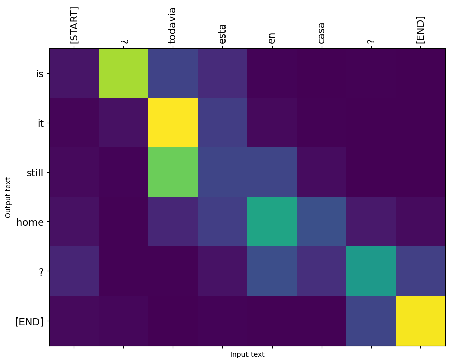
Przetłumacz jeszcze kilka zdań i wykreśl je:
%%time
three_input_text = tf.constant([
    # This is my life.
    'Esta es mi vida.',
    # Are they still home?
    '¿Todavía están en casa?',
    # Try to find out.'
    'Tratar de descubrir.',
])

result = translator.tf_translate(three_input_text)

for tr in result['text']:
  print(tr.numpy().decode())

print()
this is my life .
are you still at home ?
all about killed .

CPU times: user 78 ms, sys: 23 ms, total: 101 ms
Wall time: 23.1 ms
result['text']
<tf.Tensor: shape=(3,), dtype=string, numpy=
array([b'this is my life .', b'are you still at home ?',
       b'all about killed .'], dtype=object)>
i = 0
plot_attention(result['attention'][i], three_input_text[i], result['text'][i])
/tmpfs/src/tf_docs_env/lib/python3.7/site-packages/ipykernel_launcher.py:14: UserWarning: FixedFormatter should only be used together with FixedLocator

/tmpfs/src/tf_docs_env/lib/python3.7/site-packages/ipykernel_launcher.py:15: UserWarning: FixedFormatter should only be used together with FixedLocator
  from ipykernel import kernelapp as app

i = 1
plot_attention(result['attention'][i], three_input_text[i], result['text'][i])
/tmpfs/src/tf_docs_env/lib/python3.7/site-packages/ipykernel_launcher.py:14: UserWarning: FixedFormatter should only be used together with FixedLocator

/tmpfs/src/tf_docs_env/lib/python3.7/site-packages/ipykernel_launcher.py:15: UserWarning: FixedFormatter should only be used together with FixedLocator
  from ipykernel import kernelapp as app

i = 2
plot_attention(result['attention'][i], three_input_text[i], result['text'][i])
/tmpfs/src/tf_docs_env/lib/python3.7/site-packages/ipykernel_launcher.py:14: UserWarning: FixedFormatter should only be used together with FixedLocator

/tmpfs/src/tf_docs_env/lib/python3.7/site-packages/ipykernel_launcher.py:15: UserWarning: FixedFormatter should only be used together with FixedLocator
  from ipykernel import kernelapp as app

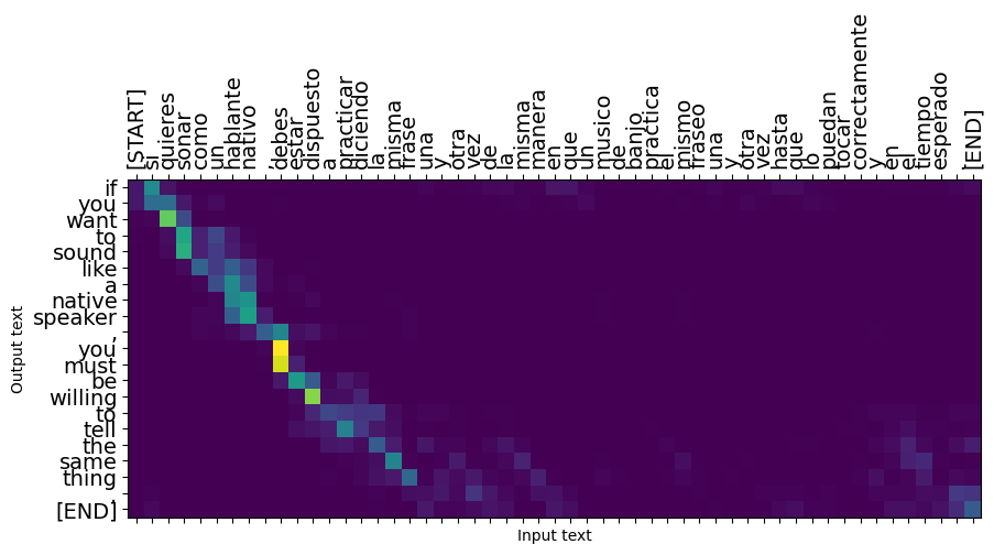
Krótkie zdania często działają dobrze, ale jeśli dane wejściowe są zbyt długie, model dosłownie traci ostrość i przestaje dostarczać rozsądnych przewidywań. Istnieją dwa główne powody takiego stanu rzeczy:
- Model został wytrenowany z wymuszaniem przez nauczyciela podawania prawidłowego tokena na każdym kroku, niezależnie od przewidywań modelu. Model mógłby być bardziej niezawodny, gdyby czasami był zasilany własnymi przewidywaniami.
- Model ma dostęp do swoich poprzednich danych wyjściowych tylko przez stan RNN. Jeśli stan RNN ulegnie uszkodzeniu, nie ma możliwości odzyskania modelu. Transformatory rozwiązać ten problem za pomocą siebie uwagę w koder i dekoder.
long_input_text = tf.constant([inp[-1]])

import textwrap
print('Expected output:\n', '\n'.join(textwrap.wrap(targ[-1])))
Expected output:
 If you want to sound like a native speaker, you must be willing to
practice saying the same sentence over and over in the same way that
banjo players practice the same phrase over and over until they can
play it correctly and at the desired tempo.
result = translator.tf_translate(long_input_text)

i = 0
plot_attention(result['attention'][i], long_input_text[i], result['text'][i])
_ = plt.suptitle('This never works')
/tmpfs/src/tf_docs_env/lib/python3.7/site-packages/ipykernel_launcher.py:14: UserWarning: FixedFormatter should only be used together with FixedLocator

/tmpfs/src/tf_docs_env/lib/python3.7/site-packages/ipykernel_launcher.py:15: UserWarning: FixedFormatter should only be used together with FixedLocator
  from ipykernel import kernelapp as app
Eksport
Gdy masz model jesteś zadowolony z was może chcieć je wyeksportować jako tf.saved_model do stosowania na zewnątrz tego programu Pythona, który go stworzył.
Ponieważ model jest podklasą tf.Module (poprzez keras.Model ), a cała funkcjonalność eksportu jest skompilowany w tf.function model powinien eksportować czysto z tf.saved_model.save :
Teraz, że funkcja została prześledzić można eksportować za pomocą saved_model.save :
tf.saved_model.save(translator, 'translator',
                    signatures={'serving_default': translator.tf_translate})
2021-12-04 12:27:54.310890: W tensorflow/python/util/util.cc:368] Sets are not currently considered sequences, but this may change in the future, so consider avoiding using them.
WARNING:absl:Found untraced functions such as encoder_2_layer_call_fn, encoder_2_layer_call_and_return_conditional_losses, decoder_2_layer_call_fn, decoder_2_layer_call_and_return_conditional_losses, embedding_4_layer_call_fn while saving (showing 5 of 60). These functions will not be directly callable after loading.
INFO:tensorflow:Assets written to: translator/assets
INFO:tensorflow:Assets written to: translator/assets
reloaded = tf.saved_model.load('translator')
result = reloaded.tf_translate(three_input_text)
%%time
result = reloaded.tf_translate(three_input_text)

for tr in result['text']:
  print(tr.numpy().decode())

print()
this is my life .
are you still at home ?
find out about to find out .

CPU times: user 42.8 ms, sys: 7.69 ms, total: 50.5 ms
Wall time: 20 ms
Następne kroki
- Pobierz inny zestaw danych do eksperymentu z tłumaczeniem na przykład z angielskiego na niemiecki, angielski lub francuski.
- Eksperymentuj z trenowaniem na większym zbiorze danych lub przy użyciu większej liczby epok.
- Spróbuj transformator poradnik , który realizuje podobne zadanie translacji ale używa warstwy transformatora zamiast RNNs. Ta wersja wykorzystuje również
text.BertTokenizerwdrożyć wordpiece tokenizacja. - Wystarczy popatrzeć na tensorflow_addons.seq2seq wdrażania tego rodzaju sekwencji modelu sekwencji.
tfa.seq2seqpakiet zawiera funkcje wyższego poziomu, npseq2seq.BeamSearchDecoder.