
 在 GitHub 上查看源代码 在 GitHub 上查看源代码 |
本笔记演示了使用条件 GAN 进行的未配对图像到图像转换,如使用循环一致的对抗网络进行未配对图像到图像转换 中所述,也称之为 CycleGAN。论文提出了一种可以捕捉图像域特征并找出如何将这些特征转换为另一个图像域的方法,而无需任何成对的训练样本。
本笔记假定您熟悉 Pix2Pix,您可以在 Pix2Pix 教程中了解有关它的信息。CycleGAN 的代码与其相似,主要区别在于额外的损失函数,以及非配对训练数据的使用。
CycleGAN 使用循环一致损失来使训练过程无需配对数据。换句话说,它可以从一个域转换到另一个域,而不需要在源域与目标域之间进行一对一映射。
这为完成许多有趣的任务开辟了可能性,例如照片增强、图片着色、风格迁移等。您所需要的只是源数据集和目标数据集(仅仅是图片目录)
设定输入管线
安装 tensorflow_examples 包,以导入生成器和判别器。
pip install git+https://github.com/tensorflow/examples.gitimport tensorflow as tf
2023-11-07 20:49:48.541969: E external/local_xla/xla/stream_executor/cuda/cuda_dnn.cc:9261] Unable to register cuDNN factory: Attempting to register factory for plugin cuDNN when one has already been registered
2023-11-07 20:49:48.542012: E external/local_xla/xla/stream_executor/cuda/cuda_fft.cc:607] Unable to register cuFFT factory: Attempting to register factory for plugin cuFFT when one has already been registered
2023-11-07 20:49:48.543716: E external/local_xla/xla/stream_executor/cuda/cuda_blas.cc:1515] Unable to register cuBLAS factory: Attempting to register factory for plugin cuBLAS when one has already been registered
import tensorflow_datasets as tfds
from tensorflow_examples.models.pix2pix import pix2pix

import os
import time
import matplotlib.pyplot as plt
from IPython.display import clear_output

AUTOTUNE = tf.data.AUTOTUNE
输入管线
本教程训练一个模型,以将普通马图片转换为斑马图片。您可以在此处获取该数据集以及类似数据集。
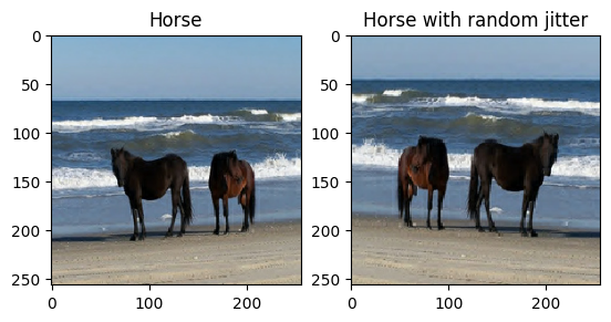
如论文所述,将随机抖动和镜像应用到训练集。这是一些避免过拟合的图像增强技术。
这类似于 pix2pix 中所做的工作。
- 在随机抖动中,图片大小调整为
286 x 286,随后被随机裁剪为256 x 256。 - 在随机镜像中,图像被水平(即从左到右)随机翻转。
dataset, metadata = tfds.load('cycle_gan/horse2zebra',
                              with_info=True, as_supervised=True)

train_horses, train_zebras = dataset['trainA'], dataset['trainB']
test_horses, test_zebras = dataset['testA'], dataset['testB']
BUFFER_SIZE = 1000
BATCH_SIZE = 1
IMG_WIDTH = 256
IMG_HEIGHT = 256
def random_crop(image):
  cropped_image = tf.image.random_crop(
      image, size=[IMG_HEIGHT, IMG_WIDTH, 3])

  return cropped_image
# normalizing the images to [-1, 1]
def normalize(image):
  image = tf.cast(image, tf.float32)
  image = (image / 127.5) - 1
  return image
def random_jitter(image):
  # resizing to 286 x 286 x 3
  image = tf.image.resize(image, [286, 286],
                          method=tf.image.ResizeMethod.NEAREST_NEIGHBOR)

  # randomly cropping to 256 x 256 x 3
  image = random_crop(image)

  # random mirroring
  image = tf.image.random_flip_left_right(image)

  return image
def preprocess_image_train(image, label):
  image = random_jitter(image)
  image = normalize(image)
  return image
def preprocess_image_test(image, label):
  image = normalize(image)
  return image
train_horses = train_horses.cache().map(
    preprocess_image_train, num_parallel_calls=AUTOTUNE).shuffle(
    BUFFER_SIZE).batch(BATCH_SIZE)

train_zebras = train_zebras.cache().map(
    preprocess_image_train, num_parallel_calls=AUTOTUNE).shuffle(
    BUFFER_SIZE).batch(BATCH_SIZE)

test_horses = test_horses.map(
    preprocess_image_test, num_parallel_calls=AUTOTUNE).cache().shuffle(
    BUFFER_SIZE).batch(BATCH_SIZE)

test_zebras = test_zebras.map(
    preprocess_image_test, num_parallel_calls=AUTOTUNE).cache().shuffle(
    BUFFER_SIZE).batch(BATCH_SIZE)
sample_horse = next(iter(train_horses))
sample_zebra = next(iter(train_zebras))
2023-11-07 20:49:55.656250: W tensorflow/core/kernels/data/cache_dataset_ops.cc:858] The calling iterator did not fully read the dataset being cached. In order to avoid unexpected truncation of the dataset, the partially cached contents of the dataset  will be discarded. This can happen if you have an input pipeline similar to `dataset.cache().take(k).repeat()`. You should use `dataset.take(k).cache().repeat()` instead.
2023-11-07 20:49:56.609214: W tensorflow/core/kernels/data/cache_dataset_ops.cc:858] The calling iterator did not fully read the dataset being cached. In order to avoid unexpected truncation of the dataset, the partially cached contents of the dataset  will be discarded. This can happen if you have an input pipeline similar to `dataset.cache().take(k).repeat()`. You should use `dataset.take(k).cache().repeat()` instead.
plt.subplot(121)
plt.title('Horse')
plt.imshow(sample_horse[0] * 0.5 + 0.5)

plt.subplot(122)
plt.title('Horse with random jitter')
plt.imshow(random_jitter(sample_horse[0]) * 0.5 + 0.5)
<matplotlib.image.AxesImage at 0x7f0344099f70>
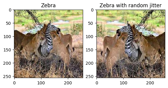
plt.subplot(121)
plt.title('Zebra')
plt.imshow(sample_zebra[0] * 0.5 + 0.5)

plt.subplot(122)
plt.title('Zebra with random jitter')
plt.imshow(random_jitter(sample_zebra[0]) * 0.5 + 0.5)
<matplotlib.image.AxesImage at 0x7f02d0157850>
导入并重用 Pix2Pix 模型
通过安装的 tensorflow_examples 包导入 Pix2Pix 中的生成器和判别器。
本教程中使用模型体系结构与 pix2pix 中所使用的非常相似。一些区别在于:
- Cyclegan 使用 instance normalization(实例归一化)而不是 batch normalization (批归一化)。
- CycleGAN 论文使用一种基于
resnet的改进生成器。简单起见,本教程使用的是改进的unet生成器。
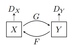
这里训练了两个生成器(G 和 F)以及两个判别器(X 和 Y)。
- 生成器
G学习将图片X转换为Y。 \((G: X -> Y)\) - 生成器
F学习将图片Y转换为X。 \((F: Y -> X)\) - 判别器
D_X学习区分图片X与生成的图片X(F(Y))。 - 判别器
D_Y学习区分图片Y与生成的图片Y(G(X))。
OUTPUT_CHANNELS = 3

generator_g = pix2pix.unet_generator(OUTPUT_CHANNELS, norm_type='instancenorm')
generator_f = pix2pix.unet_generator(OUTPUT_CHANNELS, norm_type='instancenorm')

discriminator_x = pix2pix.discriminator(norm_type='instancenorm', target=False)
discriminator_y = pix2pix.discriminator(norm_type='instancenorm', target=False)
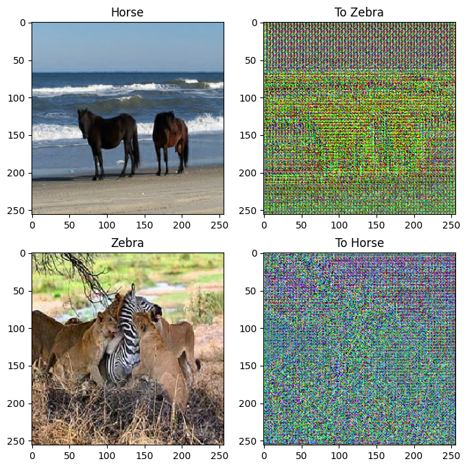
to_zebra = generator_g(sample_horse)
to_horse = generator_f(sample_zebra)
plt.figure(figsize=(8, 8))
contrast = 8

imgs = [sample_horse, to_zebra, sample_zebra, to_horse]
title = ['Horse', 'To Zebra', 'Zebra', 'To Horse']

for i in range(len(imgs)):
  plt.subplot(2, 2, i+1)
  plt.title(title[i])
  if i % 2 == 0:
    plt.imshow(imgs[i][0] * 0.5 + 0.5)
  else:
    plt.imshow(imgs[i][0] * 0.5 * contrast + 0.5)
plt.show()
WARNING:matplotlib.image:Clipping input data to the valid range for imshow with RGB data ([0..1] for floats or [0..255] for integers).
WARNING:matplotlib.image:Clipping input data to the valid range for imshow with RGB data ([0..1] for floats or [0..255] for integers).
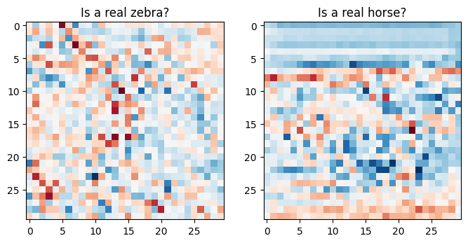
plt.figure(figsize=(8, 8))

plt.subplot(121)
plt.title('Is a real zebra?')
plt.imshow(discriminator_y(sample_zebra)[0, ..., -1], cmap='RdBu_r')

plt.subplot(122)
plt.title('Is a real horse?')
plt.imshow(discriminator_x(sample_horse)[0, ..., -1], cmap='RdBu_r')

plt.show()
损失函数
在 CycleGAN 中,没有可训练的成对数据,因此无法保证输入 x 和 目标 y 数据对在训练期间是有意义的。所以为了强制网络学习正确的映射,作者提出了循环一致损失。
判别器损失和生成器损失和 pix2pix 中所使用的类似。
LAMBDA = 10
loss_obj = tf.keras.losses.BinaryCrossentropy(from_logits=True)
def discriminator_loss(real, generated):
  real_loss = loss_obj(tf.ones_like(real), real)

  generated_loss = loss_obj(tf.zeros_like(generated), generated)

  total_disc_loss = real_loss + generated_loss

  return total_disc_loss * 0.5
def generator_loss(generated):
  return loss_obj(tf.ones_like(generated), generated)
循环一致意味着结果应接近原始输出。例如,将一句英文译为法文,随后再从法文翻译回英文,最终的结果句应与原始句输入相同。
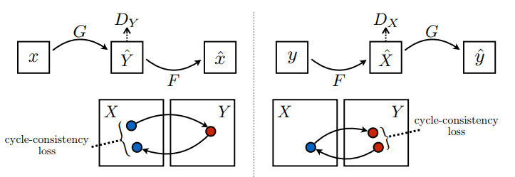
在循环一致损失中,
- 图片 \(X\) 通过生成器 \(G\) 传递,该生成器生成图片 \(\hat{Y}\)。
- 生成的图片 \(\hat{Y}\) 通过生成器 \(F\) 传递,循环生成图片 \(\hat{X}\)。
- 在 \(X\) 和 \(\hat{X}\) 之间计算平均绝对误差。
\[forward\ cycle\ consistency\ loss: X -> G(X) -> F(G(X)) \sim \hat{X}\]
\[backward\ cycle\ consistency\ loss: Y -> F(Y) -> G(F(Y)) \sim \hat{Y}\]
def calc_cycle_loss(real_image, cycled_image):
  loss1 = tf.reduce_mean(tf.abs(real_image - cycled_image))

  return LAMBDA * loss1
如上所示,生成器 \(G\) 负责将图片 \(X\) 转换为 \(Y\)。一致性损失表明,如果您将图片 \(Y\) 馈送给生成器 \(G\),它应当生成真实图片 \(Y\) 或接近于 \(Y\) 的图片。
\[Identity\ loss = |G(Y) - Y| + |F(X) - X|\]
\[Identity\ loss = |G(Y) - Y| + |F(X) - X|\]
def identity_loss(real_image, same_image):
  loss = tf.reduce_mean(tf.abs(real_image - same_image))
  return LAMBDA * 0.5 * loss
为所有生成器和判别器初始化优化器。
generator_g_optimizer = tf.keras.optimizers.Adam(2e-4, beta_1=0.5)
generator_f_optimizer = tf.keras.optimizers.Adam(2e-4, beta_1=0.5)

discriminator_x_optimizer = tf.keras.optimizers.Adam(2e-4, beta_1=0.5)
discriminator_y_optimizer = tf.keras.optimizers.Adam(2e-4, beta_1=0.5)
Checkpoints
checkpoint_path = "./checkpoints/train"

ckpt = tf.train.Checkpoint(generator_g=generator_g,
                           generator_f=generator_f,
                           discriminator_x=discriminator_x,
                           discriminator_y=discriminator_y,
                           generator_g_optimizer=generator_g_optimizer,
                           generator_f_optimizer=generator_f_optimizer,
                           discriminator_x_optimizer=discriminator_x_optimizer,
                           discriminator_y_optimizer=discriminator_y_optimizer)

ckpt_manager = tf.train.CheckpointManager(ckpt, checkpoint_path, max_to_keep=5)

# if a checkpoint exists, restore the latest checkpoint.
if ckpt_manager.latest_checkpoint:
  ckpt.restore(ckpt_manager.latest_checkpoint)
  print ('Latest checkpoint restored!!')
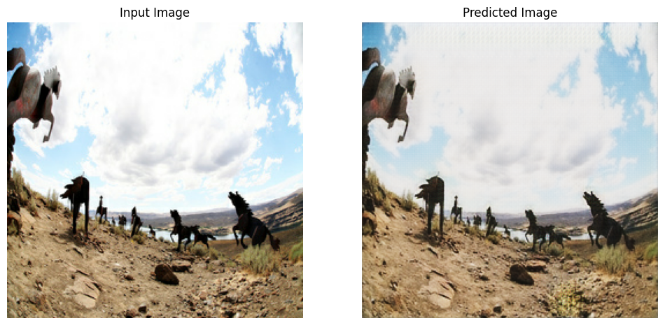
训练
注:此示例模型的训练周期 (10) 少于论文 (200),以保持本教程的训练时间合理。生成的图像质量会低得多。
EPOCHS = 10
def generate_images(model, test_input):
  prediction = model(test_input)

  plt.figure(figsize=(12, 12))

  display_list = [test_input[0], prediction[0]]
  title = ['Input Image', 'Predicted Image']

  for i in range(2):
    plt.subplot(1, 2, i+1)
    plt.title(title[i])
    # getting the pixel values between [0, 1] to plot it.
    plt.imshow(display_list[i] * 0.5 + 0.5)
    plt.axis('off')
  plt.show()
尽管训练循环看起来很复杂,其实包含四个基本步骤:
- 获取预测。
- 计算损失值。
- 使用反向传播计算损失值。
- 将梯度应用于优化器。
@tf.function
def train_step(real_x, real_y):
  # persistent is set to True because the tape is used more than
  # once to calculate the gradients.
  with tf.GradientTape(persistent=True) as tape:
    # Generator G translates X -> Y
    # Generator F translates Y -> X.

    fake_y = generator_g(real_x, training=True)
    cycled_x = generator_f(fake_y, training=True)

    fake_x = generator_f(real_y, training=True)
    cycled_y = generator_g(fake_x, training=True)

    # same_x and same_y are used for identity loss.
    same_x = generator_f(real_x, training=True)
    same_y = generator_g(real_y, training=True)

    disc_real_x = discriminator_x(real_x, training=True)
    disc_real_y = discriminator_y(real_y, training=True)

    disc_fake_x = discriminator_x(fake_x, training=True)
    disc_fake_y = discriminator_y(fake_y, training=True)

    # calculate the loss
    gen_g_loss = generator_loss(disc_fake_y)
    gen_f_loss = generator_loss(disc_fake_x)

    total_cycle_loss = calc_cycle_loss(real_x, cycled_x) + calc_cycle_loss(real_y, cycled_y)

    # Total generator loss = adversarial loss + cycle loss
    total_gen_g_loss = gen_g_loss + total_cycle_loss + identity_loss(real_y, same_y)
    total_gen_f_loss = gen_f_loss + total_cycle_loss + identity_loss(real_x, same_x)

    disc_x_loss = discriminator_loss(disc_real_x, disc_fake_x)
    disc_y_loss = discriminator_loss(disc_real_y, disc_fake_y)

  # Calculate the gradients for generator and discriminator
  generator_g_gradients = tape.gradient(total_gen_g_loss,
                                        generator_g.trainable_variables)
  generator_f_gradients = tape.gradient(total_gen_f_loss,
                                        generator_f.trainable_variables)

  discriminator_x_gradients = tape.gradient(disc_x_loss,
                                            discriminator_x.trainable_variables)
  discriminator_y_gradients = tape.gradient(disc_y_loss,
                                            discriminator_y.trainable_variables)

  # Apply the gradients to the optimizer
  generator_g_optimizer.apply_gradients(zip(generator_g_gradients,
                                            generator_g.trainable_variables))

  generator_f_optimizer.apply_gradients(zip(generator_f_gradients,
                                            generator_f.trainable_variables))

  discriminator_x_optimizer.apply_gradients(zip(discriminator_x_gradients,
                                                discriminator_x.trainable_variables))

  discriminator_y_optimizer.apply_gradients(zip(discriminator_y_gradients,
                                                discriminator_y.trainable_variables))
for epoch in range(EPOCHS):
  start = time.time()

  n = 0
  for image_x, image_y in tf.data.Dataset.zip((train_horses, train_zebras)):
    train_step(image_x, image_y)
    if n % 10 == 0:
      print ('.', end='')
    n += 1

  clear_output(wait=True)
  # Using a consistent image (sample_horse) so that the progress of the model
  # is clearly visible.
  generate_images(generator_g, sample_horse)

  if (epoch + 1) % 5 == 0:
    ckpt_save_path = ckpt_manager.save()
    print ('Saving checkpoint for epoch {} at {}'.format(epoch+1,
                                                         ckpt_save_path))

  print ('Time taken for epoch {} is {} sec\n'.format(epoch + 1,
                                                      time.time()-start))
Saving checkpoint for epoch 10 at ./checkpoints/train/ckpt-2
Time taken for epoch 10 is 466.6620719432831 sec
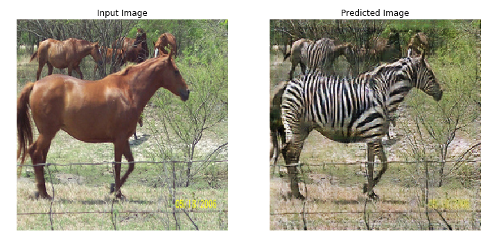
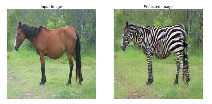
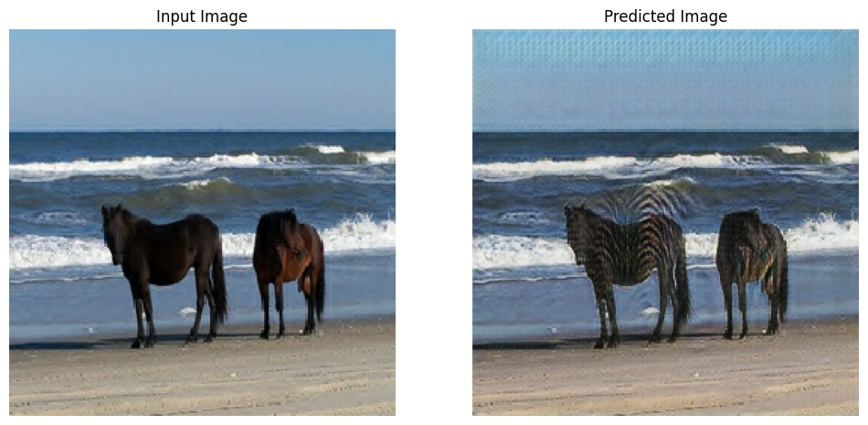
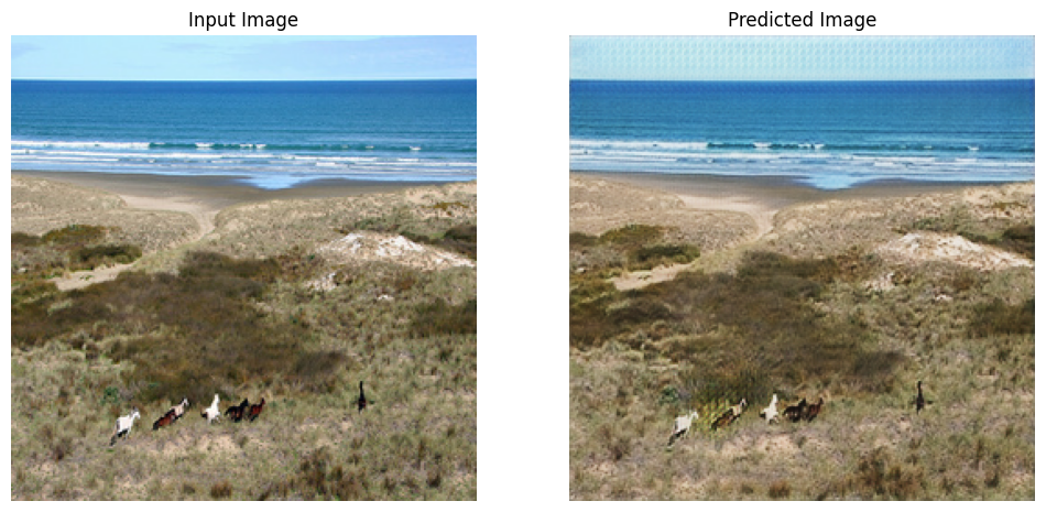
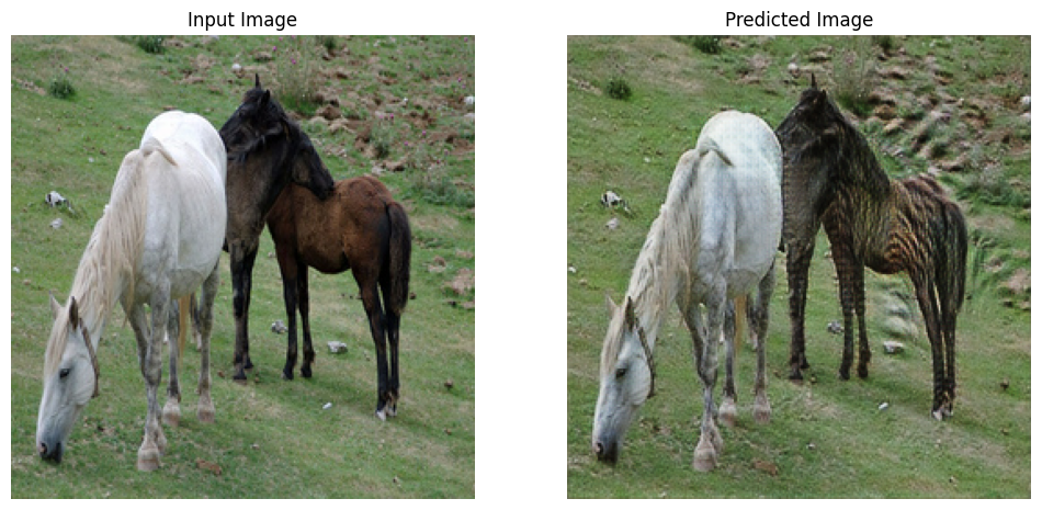
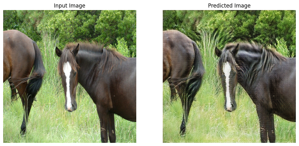
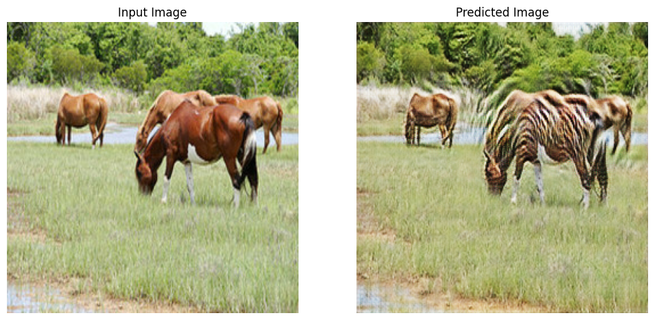
使用测试数据集进行生成
# Run the trained model on the test dataset
for inp in test_horses.take(5):
  generate_images(generator_g, inp)
下一步
本教程展示了如何从 Pix2Pix 教程实现的生成器和判别器开始实现 CycleGAN。 下一步,您可以尝试使用一个来源于 TensorFlow 数据集的不同的数据集。
您也可以训练更多的 epoch 以改进结果,或者可以实现论文中所使用的改进 ResNet 生成器来代替这里使用的 U-Net 生成器。