
| | |  GitHub पर स्रोत देखें GitHub पर स्रोत देखें | |
यह ट्यूटोरियल Tensorflow फ़ेडरेटेड का उपयोग करके उपयोगकर्ता-स्तरीय डिफरेंशियल प्राइवेसी के साथ प्रशिक्षण मॉडल के लिए अनुशंसित सर्वोत्तम अभ्यास प्रदर्शित करेगा। हम डी पी-SGD एल्गोरिथ्म का उपयोग करेगा Abadi एट अल।, "विभेदक गोपनीयता के साथ दीप लर्निंग" में एक फ़ेडरेटेड संदर्भ में उपयोगकर्ता के स्तर डी पी के लिए संशोधित McMahan एट अल।, "सीखना भिन्न निजी बारम्बार भाषा मॉडल" ।
डिफरेंशियल प्राइवेसी (डीपी) सीखने के कार्यों को करते समय संवेदनशील डेटा की गोपनीयता रिसाव को सीमित करने और मापने के लिए व्यापक रूप से उपयोग की जाने वाली विधि है। उपयोगकर्ता-स्तर डीपी के साथ एक मॉडल का प्रशिक्षण गारंटी देता है कि मॉडल किसी भी व्यक्ति के डेटा के बारे में कुछ भी महत्वपूर्ण सीखने की संभावना नहीं है, लेकिन फिर भी (उम्मीद है!) कई ग्राहकों के डेटा में मौजूद पैटर्न सीख सकता है।
हम फ़ेडरेटेड EMNIST डेटासेट पर एक मॉडल को प्रशिक्षित करेंगे। उपयोगिता और गोपनीयता के बीच एक अंतर्निहित व्यापार-बंद है, और उच्च गोपनीयता वाले मॉडल को प्रशिक्षित करना मुश्किल हो सकता है जो एक अत्याधुनिक गैर-निजी मॉडल के साथ-साथ प्रदर्शन करता है। इस ट्यूटोरियल में शीघ्रता के लिए, हम उच्च गोपनीयता के साथ प्रशिक्षित करने के तरीके को प्रदर्शित करने के लिए कुछ गुणवत्ता का त्याग करते हुए, केवल 100 राउंड के लिए प्रशिक्षण देंगे। यदि हम अधिक प्रशिक्षण दौर का उपयोग करते हैं, तो हमारे पास निश्चित रूप से कुछ हद तक उच्च सटीकता वाला निजी मॉडल हो सकता है, लेकिन डीपी के बिना प्रशिक्षित मॉडल जितना ऊंचा नहीं होगा।
इससे पहले कि हम शुरू करें
सबसे पहले, आइए सुनिश्चित करें कि नोटबुक एक बैकएंड से जुड़ा है जिसमें प्रासंगिक घटक संकलित हैं।
!pip install --quiet --upgrade tensorflow_federated_nightly
!pip install --quiet --upgrade nest-asyncio

import nest_asyncio
nest_asyncio.apply()
कुछ आयातों की हमें ट्यूटोरियल के लिए आवश्यकता होगी। हम उपयोग करेगा tensorflow_federated , मशीन सीखने और विकेंद्रीकरण डेटा पर अन्य संगणना, साथ ही के लिए खुला स्रोत ढांचे tensorflow_privacy , लागू करने और tensorflow में भिन्न निजी एल्गोरिदम विश्लेषण करने के लिए खुला स्रोत पुस्तकालय।
import collections

import numpy as np
import pandas as pd
import tensorflow as tf
import tensorflow_federated as tff
import tensorflow_privacy as tfp
यह सुनिश्चित करने के लिए कि TFF वातावरण सही ढंग से सेटअप है, निम्नलिखित "हैलो वर्ल्ड" उदाहरण चलाएँ। यह काम नहीं करता है, तो कृपया स्थापना निर्देश के लिए गाइड।
@tff.federated_computation
def hello_world():
  return 'Hello, World!'

hello_world()
b'Hello, World!'
फ़ेडरेटेड EMNIST डेटासेट डाउनलोड करें और प्रीप्रोसेस करें।
def get_emnist_dataset():
  emnist_train, emnist_test = tff.simulation.datasets.emnist.load_data(
      only_digits=True)

  def element_fn(element):
    return collections.OrderedDict(
        x=tf.expand_dims(element['pixels'], -1), y=element['label'])

  def preprocess_train_dataset(dataset):
    # Use buffer_size same as the maximum client dataset size,
    # 418 for Federated EMNIST
    return (dataset.map(element_fn)
                   .shuffle(buffer_size=418)
                   .repeat(1)
                   .batch(32, drop_remainder=False))

  def preprocess_test_dataset(dataset):
    return dataset.map(element_fn).batch(128, drop_remainder=False)

  emnist_train = emnist_train.preprocess(preprocess_train_dataset)
  emnist_test = preprocess_test_dataset(
      emnist_test.create_tf_dataset_from_all_clients())
  return emnist_train, emnist_test

train_data, test_data = get_emnist_dataset()
हमारे मॉडल को परिभाषित करें।
def my_model_fn():
  model = tf.keras.models.Sequential([
      tf.keras.layers.Reshape(input_shape=(28, 28, 1), target_shape=(28 * 28,)),
      tf.keras.layers.Dense(200, activation=tf.nn.relu),
      tf.keras.layers.Dense(200, activation=tf.nn.relu),
      tf.keras.layers.Dense(10)])
  return tff.learning.from_keras_model(
      keras_model=model,
      loss=tf.keras.losses.SparseCategoricalCrossentropy(from_logits=True),
      input_spec=test_data.element_spec,
      metrics=[tf.keras.metrics.SparseCategoricalAccuracy()])
मॉडल की शोर संवेदनशीलता का निर्धारण करें।
उपयोगकर्ता-स्तरीय डीपी गारंटी प्राप्त करने के लिए, हमें बुनियादी फ़ेडरेटेड एवरेजिंग एल्गोरिथम को दो तरीकों से बदलना होगा। सबसे पहले, क्लाइंट के मॉडल अपडेट को सर्वर पर ट्रांसमिशन से पहले क्लिप किया जाना चाहिए, जिससे किसी एक क्लाइंट के अधिकतम प्रभाव को सीमित किया जा सके। दूसरा, सर्वर को सबसे खराब स्थिति वाले क्लाइंट प्रभाव को अस्पष्ट करने के लिए औसत से पहले उपयोगकर्ता अपडेट के योग में पर्याप्त शोर जोड़ना चाहिए।
कतरन के लिए, हम के अनुकूली कतरन विधि का उपयोग एंड्रयू एट अल। 2021, अनुकूली कतरन के साथ भिन्न निजी लर्निंग , स्पष्ट रूप से सेट किया जा करने के लिए कोई कतरन आदर्श की जरूरत है तो।
शोर जोड़ने से सामान्य रूप से मॉडल की उपयोगिता कम हो जाएगी, लेकिन हम प्रत्येक दौर में दो नॉब्स के साथ औसत अपडेट में शोर की मात्रा को नियंत्रित कर सकते हैं: गॉसियन शोर का मानक विचलन योग में जोड़ा जाता है, और ग्राहकों की संख्या में औसत। हमारी रणनीति पहले यह निर्धारित करने की होगी कि मॉडल उपयोगिता को स्वीकार्य नुकसान के साथ प्रति राउंड अपेक्षाकृत कम संख्या में ग्राहकों के साथ मॉडल कितना शोर सहन कर सकता है। फिर अंतिम मॉडल को प्रशिक्षित करने के लिए, हम योग में शोर की मात्रा बढ़ा सकते हैं, जबकि आनुपातिक रूप से प्रति राउंड ग्राहकों की संख्या को बढ़ा सकते हैं (यह मानते हुए कि डेटासेट प्रति राउंड कई क्लाइंट का समर्थन करने के लिए पर्याप्त है)। यह मॉडल की गुणवत्ता को महत्वपूर्ण रूप से प्रभावित करने की संभावना नहीं है, क्योंकि क्लाइंट नमूनाकरण के कारण भिन्नता को कम करना एकमात्र प्रभाव है (वास्तव में हम सत्यापित करेंगे कि यह हमारे मामले में नहीं है)।
इसके लिए, हम पहले 50 ग्राहकों के साथ मॉडल की एक श्रृंखला को प्रशिक्षित करते हैं, जिसमें शोर की मात्रा बढ़ती है। विशेष रूप से, हम "noise_multiplier" को बढ़ाते हैं जो कि क्लिपिंग मानदंड के लिए शोर मानक विचलन का अनुपात है। चूंकि हम अनुकूली कतरन का उपयोग कर रहे हैं, इसका मतलब है कि शोर का वास्तविक परिमाण गोल से गोल में बदल जाता है।
# Run five clients per thread. Increase this if your runtime is running out of
# memory. Decrease it if you have the resources and want to speed up execution.
tff.backends.native.set_local_python_execution_context(clients_per_thread=5)

total_clients = len(train_data.client_ids)

def train(rounds, noise_multiplier, clients_per_round, data_frame):
  # Using the `dp_aggregator` here turns on differential privacy with adaptive
  # clipping.
  aggregation_factory = tff.learning.model_update_aggregator.dp_aggregator(
      noise_multiplier, clients_per_round)

  # We use Poisson subsampling which gives slightly tighter privacy guarantees
  # compared to having a fixed number of clients per round. The actual number of
  # clients per round is stochastic with mean clients_per_round.
  sampling_prob = clients_per_round / total_clients

  # Build a federated averaging process.
  # Typically a non-adaptive server optimizer is used because the noise in the
  # updates can cause the second moment accumulators to become very large
  # prematurely.
  learning_process = tff.learning.build_federated_averaging_process(
        my_model_fn,
        client_optimizer_fn=lambda: tf.keras.optimizers.SGD(0.01),
        server_optimizer_fn=lambda: tf.keras.optimizers.SGD(1.0, momentum=0.9),
        model_update_aggregation_factory=aggregation_factory)

  eval_process = tff.learning.build_federated_evaluation(my_model_fn)

  # Training loop.
  state = learning_process.initialize()
  for round in range(rounds):
    if round % 5 == 0:
      metrics = eval_process(state.model, [test_data])['eval']
      if round < 25 or round % 25 == 0:
        print(f'Round {round:3d}: {metrics}')
      data_frame = data_frame.append({'Round': round,
                                      'NoiseMultiplier': noise_multiplier,
                                      **metrics}, ignore_index=True)

    # Sample clients for a round. Note that if your dataset is large and
    # sampling_prob is small, it would be faster to use gap sampling.
    x = np.random.uniform(size=total_clients)
    sampled_clients = [
        train_data.client_ids[i] for i in range(total_clients)
        if x[i] < sampling_prob]
    sampled_train_data = [
        train_data.create_tf_dataset_for_client(client)
        for client in sampled_clients]

    # Use selected clients for update.
    state, metrics = learning_process.next(state, sampled_train_data)

  metrics = eval_process(state.model, [test_data])['eval']
  print(f'Round {rounds:3d}: {metrics}')
  data_frame = data_frame.append({'Round': rounds,
                                  'NoiseMultiplier': noise_multiplier,
                                  **metrics}, ignore_index=True)

  return data_frame
data_frame = pd.DataFrame()
rounds = 100
clients_per_round = 50

for noise_multiplier in [0.0, 0.5, 0.75, 1.0]:
  print(f'Starting training with noise multiplier: {noise_multiplier}')
  data_frame = train(rounds, noise_multiplier, clients_per_round, data_frame)
  print()
Starting training with noise multiplier: 0.0
Round   0: OrderedDict([('sparse_categorical_accuracy', 0.112289384), ('loss', 2.5190482)])
Round   5: OrderedDict([('sparse_categorical_accuracy', 0.19075724), ('loss', 2.2449977)])
Round  10: OrderedDict([('sparse_categorical_accuracy', 0.18115693), ('loss', 2.163907)])
Round  15: OrderedDict([('sparse_categorical_accuracy', 0.49970612), ('loss', 2.01017)])
Round  20: OrderedDict([('sparse_categorical_accuracy', 0.5333317), ('loss', 1.8350543)])
Round  25: OrderedDict([('sparse_categorical_accuracy', 0.5828517), ('loss', 1.6551636)])
Round  50: OrderedDict([('sparse_categorical_accuracy', 0.7352077), ('loss', 0.8700141)])
Round  75: OrderedDict([('sparse_categorical_accuracy', 0.7769152), ('loss', 0.6992781)])
Round 100: OrderedDict([('sparse_categorical_accuracy', 0.8049814), ('loss', 0.62453026)])

Starting training with noise multiplier: 0.5
Round   0: OrderedDict([('sparse_categorical_accuracy', 0.09526841), ('loss', 2.4332638)])
Round   5: OrderedDict([('sparse_categorical_accuracy', 0.20128821), ('loss', 2.2664592)])
Round  10: OrderedDict([('sparse_categorical_accuracy', 0.35472178), ('loss', 2.130336)])
Round  15: OrderedDict([('sparse_categorical_accuracy', 0.5480995), ('loss', 1.9713942)])
Round  20: OrderedDict([('sparse_categorical_accuracy', 0.42246276), ('loss', 1.8045483)])
Round  25: OrderedDict([('sparse_categorical_accuracy', 0.624902), ('loss', 1.4785467)])
Round  50: OrderedDict([('sparse_categorical_accuracy', 0.7265625), ('loss', 0.85801566)])
Round  75: OrderedDict([('sparse_categorical_accuracy', 0.77720904), ('loss', 0.70615387)])
Round 100: OrderedDict([('sparse_categorical_accuracy', 0.7702537), ('loss', 0.72331005)])

Starting training with noise multiplier: 0.75
Round   0: OrderedDict([('sparse_categorical_accuracy', 0.098672606), ('loss', 2.422002)])
Round   5: OrderedDict([('sparse_categorical_accuracy', 0.11794671), ('loss', 2.2227976)])
Round  10: OrderedDict([('sparse_categorical_accuracy', 0.3208513), ('loss', 2.083766)])
Round  15: OrderedDict([('sparse_categorical_accuracy', 0.49752644), ('loss', 1.8728142)])
Round  20: OrderedDict([('sparse_categorical_accuracy', 0.5816761), ('loss', 1.6084186)])
Round  25: OrderedDict([('sparse_categorical_accuracy', 0.62896746), ('loss', 1.378527)])
Round  50: OrderedDict([('sparse_categorical_accuracy', 0.73153406), ('loss', 0.8705139)])
Round  75: OrderedDict([('sparse_categorical_accuracy', 0.7789724), ('loss', 0.7113147)])
Round 100: OrderedDict([('sparse_categorical_accuracy', 0.70944357), ('loss', 0.89495045)])

Starting training with noise multiplier: 1.0
Round   0: OrderedDict([('sparse_categorical_accuracy', 0.12002841), ('loss', 2.60482)])
Round   5: OrderedDict([('sparse_categorical_accuracy', 0.104574844), ('loss', 2.3388205)])
Round  10: OrderedDict([('sparse_categorical_accuracy', 0.29966694), ('loss', 2.089262)])
Round  15: OrderedDict([('sparse_categorical_accuracy', 0.4067398), ('loss', 1.9109797)])
Round  20: OrderedDict([('sparse_categorical_accuracy', 0.5123677), ('loss', 1.6472703)])
Round  25: OrderedDict([('sparse_categorical_accuracy', 0.56416535), ('loss', 1.4362282)])
Round  50: OrderedDict([('sparse_categorical_accuracy', 0.62323666), ('loss', 1.1682972)])
Round  75: OrderedDict([('sparse_categorical_accuracy', 0.55968356), ('loss', 1.4779186)])
Round 100: OrderedDict([('sparse_categorical_accuracy', 0.382837), ('loss', 1.9680436)])
अब हम मूल्यांकन सेट की सटीकता और उन रनों के नुकसान की कल्पना कर सकते हैं।
import matplotlib.pyplot as plt
import seaborn as sns

def make_plot(data_frame):
  plt.figure(figsize=(15, 5))

  dff = data_frame.rename(
      columns={'sparse_categorical_accuracy': 'Accuracy', 'loss': 'Loss'})

  plt.subplot(121)
  sns.lineplot(data=dff, x='Round', y='Accuracy', hue='NoiseMultiplier', palette='dark')
  plt.subplot(122)
  sns.lineplot(data=dff, x='Round', y='Loss', hue='NoiseMultiplier', palette='dark')
make_plot(data_frame)
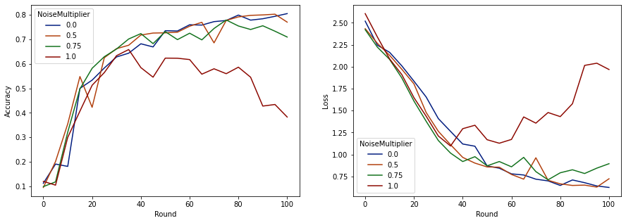
ऐसा प्रतीत होता है कि प्रति राउंड 50 अपेक्षित ग्राहकों के साथ, यह मॉडल मॉडल की गुणवत्ता में गिरावट के बिना 0.5 तक के शोर गुणक को सहन कर सकता है। 0.75 का एक शोर गुणक मॉडल के थोड़ा खराब होने का कारण बनता है, और 1.0 मॉडल को अलग कर देता है।
आमतौर पर मॉडल की गुणवत्ता और गोपनीयता के बीच एक समझौता होता है। हम जितना अधिक शोर का उपयोग करते हैं, उतनी ही अधिक गोपनीयता हम प्रशिक्षण समय और ग्राहकों की संख्या के लिए प्राप्त कर सकते हैं। इसके विपरीत, कम शोर के साथ, हमारे पास एक अधिक सटीक मॉडल हो सकता है, लेकिन हमें अपने लक्षित गोपनीयता स्तर तक पहुंचने के लिए प्रति राउंड अधिक ग्राहकों के साथ प्रशिक्षण लेना होगा।
उपरोक्त प्रयोग के साथ, हम यह तय कर सकते हैं कि अंतिम मॉडल को तेजी से प्रशिक्षित करने के लिए 0.75 पर मॉडल गिरावट की छोटी मात्रा स्वीकार्य है, लेकिन मान लें कि हम 0.5 शोर-गुणक मॉडल के प्रदर्शन से मेल खाना चाहते हैं।
अब हम tensorflow_privacy फ़ंक्शन का उपयोग यह निर्धारित करने के लिए कर सकते हैं कि स्वीकार्य गोपनीयता प्राप्त करने के लिए हमें प्रति राउंड कितने अपेक्षित क्लाइंट की आवश्यकता होगी। मानक अभ्यास यह है कि डेटासेट में रिकॉर्ड की संख्या के मुकाबले डेल्टा को एक से कुछ छोटा चुना जाए। इस डेटासेट में कुल 3383 प्रशिक्षण उपयोगकर्ता हैं, तो चलिए (2, 1e-5)-DP का लक्ष्य रखते हैं।
हम प्रति राउंड क्लाइंट्स की संख्या पर एक साधारण बाइनरी सर्च का उपयोग करते हैं। Tensorflow_privacy समारोह हम एप्सिलॉन अनुमान लगाने के लिए उपयोग करने पर आधारित है वांग एट अल। (2018) और मिरोनोव एट अल। (2019) ।
rdp_orders = ([1.25, 1.5, 1.75, 2., 2.25, 2.5, 3., 3.5, 4., 4.5] +
              list(range(5, 64)) + [128, 256, 512])

total_clients = 3383
base_noise_multiplier = 0.5
base_clients_per_round = 50
target_delta = 1e-5
target_eps = 2

def get_epsilon(clients_per_round):
  # If we use this number of clients per round and proportionally
  # scale up the noise multiplier, what epsilon do we achieve?
  q = clients_per_round / total_clients
  noise_multiplier = base_noise_multiplier
  noise_multiplier *= clients_per_round / base_clients_per_round
  rdp = tfp.compute_rdp(
      q, noise_multiplier=noise_multiplier, steps=rounds, orders=rdp_orders)
  eps, _, _ = tfp.get_privacy_spent(rdp_orders, rdp, target_delta=target_delta)
  return clients_per_round, eps, noise_multiplier

def find_needed_clients_per_round():
  hi = get_epsilon(base_clients_per_round)
  if hi[1] < target_eps:
    return hi

  # Grow interval exponentially until target_eps is exceeded.
  while True:
    lo = hi
    hi = get_epsilon(2 * lo[0])
    if hi[1] < target_eps:
      break

  # Binary search.
  while hi[0] - lo[0] > 1:
    mid = get_epsilon((lo[0] + hi[0]) // 2)
    if mid[1] > target_eps:
      lo = mid
    else:
      hi = mid

  return hi

clients_per_round, _, noise_multiplier = find_needed_clients_per_round()
print(f'To get ({target_eps}, {target_delta})-DP, use {clients_per_round} '
      f'clients with noise multiplier {noise_multiplier}.')
To get (2, 1e-05)-DP, use 120 clients with noise multiplier 1.2.
अब हम रिलीज के लिए अपने अंतिम निजी मॉडल को प्रशिक्षित कर सकते हैं।
rounds = 100
noise_multiplier = 1.2
clients_per_round = 120

data_frame = pd.DataFrame()
data_frame = train(rounds, noise_multiplier, clients_per_round, data_frame)

make_plot(data_frame)
Round   0: OrderedDict([('sparse_categorical_accuracy', 0.08260678), ('loss', 2.6334999)])
Round   5: OrderedDict([('sparse_categorical_accuracy', 0.1492212), ('loss', 2.259542)])
Round  10: OrderedDict([('sparse_categorical_accuracy', 0.28847474), ('loss', 2.155699)])
Round  15: OrderedDict([('sparse_categorical_accuracy', 0.3989518), ('loss', 2.0156953)])
Round  20: OrderedDict([('sparse_categorical_accuracy', 0.5086697), ('loss', 1.8261365)])
Round  25: OrderedDict([('sparse_categorical_accuracy', 0.6204692), ('loss', 1.5602393)])
Round  50: OrderedDict([('sparse_categorical_accuracy', 0.70008814), ('loss', 0.91155165)])
Round  75: OrderedDict([('sparse_categorical_accuracy', 0.78421336), ('loss', 0.6820159)])
Round 100: OrderedDict([('sparse_categorical_accuracy', 0.7955525), ('loss', 0.6585961)])
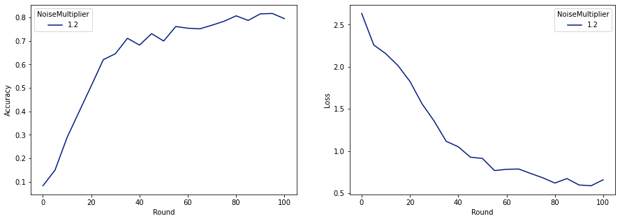
जैसा कि हम देख सकते हैं, अंतिम मॉडल में बिना शोर के प्रशिक्षित मॉडल के समान नुकसान और सटीकता है, लेकिन यह (2, 1e-5) -DP को संतुष्ट करता है।