
| | |  Voir la source sur GitHub Voir la source sur GitHub | |
Aperçu
L'API tf.distribute.Strategy fournit une abstraction pour la distribution de votre formation sur plusieurs unités de traitement. Il vous permet d'effectuer une formation distribuée à l'aide de modèles et de code de formation existants avec un minimum de modifications.
Ce didacticiel montre comment utiliser tf.distribute.MirroredStrategy pour effectuer une réplication dans le graphique avec une formation synchrone sur plusieurs GPU sur une seule machine . La stratégie copie essentiellement toutes les variables du modèle sur chaque processeur. Ensuite, il utilise all-reduce pour combiner les gradients de tous les processeurs et applique la valeur combinée à toutes les copies du modèle.
Vous utiliserez les API tf.keras pour créer le modèle et Model.fit pour l'entraîner. (Pour en savoir plus sur la formation distribuée avec une boucle de formation personnalisée et la MirroredStrategy , consultez ce didacticiel .)
MirroredStrategy entraîne votre modèle sur plusieurs GPU sur une seule machine. Pour une formation synchrone sur plusieurs GPU sur plusieurs nœuds de calcul, utilisez tf.distribute.MultiWorkerMirroredStrategy avec Keras Model.fit ou une boucle de formation personnalisée . Pour les autres options, reportez-vous au Guide de formation distribuée .
Pour en savoir plus sur diverses autres stratégies, il existe le guide Formation distribuée avec TensorFlow .
Installer
import tensorflow_datasets as tfds
import tensorflow as tf

import os

# Load the TensorBoard notebook extension.
%load_ext tensorboard
print(tf.__version__)
2.8.0-rc1
Télécharger le jeu de données
Chargez l'ensemble de données MNIST à partir de TensorFlow Datasets . Cela renvoie un ensemble de données au format tf.data .
La définition de l'argument with_info sur True inclut les métadonnées de l'ensemble de données, qui sont enregistrées ici dans info . Entre autres choses, cet objet de métadonnées comprend le nombre d'exemples d'entraînement et de test.
datasets, info = tfds.load(name='mnist', with_info=True, as_supervised=True)

mnist_train, mnist_test = datasets['train'], datasets['test']
Définir la stratégie de distribution
Créez un objet MirroredStrategy . Cela gérera la distribution et fournira un gestionnaire de contexte ( MirroredStrategy.scope ) pour construire votre modèle à l'intérieur.
strategy = tf.distribute.MirroredStrategy()
INFO:tensorflow:Using MirroredStrategy with devices ('/job:localhost/replica:0/task:0/device:GPU:0',)
INFO:tensorflow:Using MirroredStrategy with devices ('/job:localhost/replica:0/task:0/device:GPU:0',)
print('Number of devices: {}'.format(strategy.num_replicas_in_sync))
Number of devices: 1
Configurer le pipeline d'entrée
Lors de la formation d'un modèle avec plusieurs GPU, vous pouvez utiliser efficacement la puissance de calcul supplémentaire en augmentant la taille du lot. En général, utilisez la plus grande taille de lot adaptée à la mémoire GPU et réglez le taux d'apprentissage en conséquence.
# You can also do info.splits.total_num_examples to get the total
# number of examples in the dataset.

num_train_examples = info.splits['train'].num_examples
num_test_examples = info.splits['test'].num_examples

BUFFER_SIZE = 10000

BATCH_SIZE_PER_REPLICA = 64
BATCH_SIZE = BATCH_SIZE_PER_REPLICA * strategy.num_replicas_in_sync
Définissez une fonction qui normalise les valeurs des pixels de l'image de la plage [0, 255] à la plage [0, 1] (mise à l' échelle des fonctionnalités ) :
def scale(image, label):
  image = tf.cast(image, tf.float32)
  image /= 255

  return image, label
Appliquez cette fonction d' scale aux données d'entraînement et de test, puis utilisez les API tf.data.Dataset pour mélanger les données d'entraînement ( Dataset.shuffle ) et les regrouper ( Dataset.batch ). Notez que vous conservez également un cache en mémoire des données d'entraînement pour améliorer les performances ( Dataset.cache ).
train_dataset = mnist_train.map(scale).cache().shuffle(BUFFER_SIZE).batch(BATCH_SIZE)
eval_dataset = mnist_test.map(scale).batch(BATCH_SIZE)
Créer le modèle
Créer et compiler le modèle Keras dans le contexte de Strategy.scope :
with strategy.scope():
  model = tf.keras.Sequential([
      tf.keras.layers.Conv2D(32, 3, activation='relu', input_shape=(28, 28, 1)),
      tf.keras.layers.MaxPooling2D(),
      tf.keras.layers.Flatten(),
      tf.keras.layers.Dense(64, activation='relu'),
      tf.keras.layers.Dense(10)
  ])

  model.compile(loss=tf.keras.losses.SparseCategoricalCrossentropy(from_logits=True),
                optimizer=tf.keras.optimizers.Adam(),
                metrics=['accuracy'])
INFO:tensorflow:Reduce to /job:localhost/replica:0/task:0/device:CPU:0 then broadcast to ('/job:localhost/replica:0/task:0/device:CPU:0',).
INFO:tensorflow:Reduce to /job:localhost/replica:0/task:0/device:CPU:0 then broadcast to ('/job:localhost/replica:0/task:0/device:CPU:0',).
INFO:tensorflow:Reduce to /job:localhost/replica:0/task:0/device:CPU:0 then broadcast to ('/job:localhost/replica:0/task:0/device:CPU:0',).
INFO:tensorflow:Reduce to /job:localhost/replica:0/task:0/device:CPU:0 then broadcast to ('/job:localhost/replica:0/task:0/device:CPU:0',).
INFO:tensorflow:Reduce to /job:localhost/replica:0/task:0/device:CPU:0 then broadcast to ('/job:localhost/replica:0/task:0/device:CPU:0',).
INFO:tensorflow:Reduce to /job:localhost/replica:0/task:0/device:CPU:0 then broadcast to ('/job:localhost/replica:0/task:0/device:CPU:0',).
INFO:tensorflow:Reduce to /job:localhost/replica:0/task:0/device:CPU:0 then broadcast to ('/job:localhost/replica:0/task:0/device:CPU:0',).
INFO:tensorflow:Reduce to /job:localhost/replica:0/task:0/device:CPU:0 then broadcast to ('/job:localhost/replica:0/task:0/device:CPU:0',).
Définir les rappels
Définissez les tf.keras.callbacks suivants :
-
tf.keras.callbacks.TensorBoard: écrit un journal pour TensorBoard, qui permet de visualiser les graphiques. -
tf.keras.callbacks.ModelCheckpoint: enregistre le modèle à une certaine fréquence, comme après chaque époque. -
tf.keras.callbacks.LearningRateScheduler: planifie le changement du taux d'apprentissage après, par exemple, chaque époque/lot.
À des fins d'illustration, ajoutez un rappel personnalisé appelé PrintLR pour afficher le taux d'apprentissage dans le bloc-notes.
# Define the checkpoint directory to store the checkpoints.
checkpoint_dir = './training_checkpoints'
# Define the name of the checkpoint files.
checkpoint_prefix = os.path.join(checkpoint_dir, "ckpt_{epoch}")
# Define a function for decaying the learning rate.
# You can define any decay function you need.
def decay(epoch):
  if epoch < 3:
    return 1e-3
  elif epoch >= 3 and epoch < 7:
    return 1e-4
  else:
    return 1e-5
# Define a callback for printing the learning rate at the end of each epoch.
class PrintLR(tf.keras.callbacks.Callback):
  def on_epoch_end(self, epoch, logs=None):
    print('\nLearning rate for epoch {} is {}'.format(epoch + 1,
                                                      model.optimizer.lr.numpy()))
# Put all the callbacks together.
callbacks = [
    tf.keras.callbacks.TensorBoard(log_dir='./logs'),
    tf.keras.callbacks.ModelCheckpoint(filepath=checkpoint_prefix,
                                       save_weights_only=True),
    tf.keras.callbacks.LearningRateScheduler(decay),
    PrintLR()
]
Former et évaluer
Maintenant, entraînez le modèle de la manière habituelle en appelant Model.fit sur le modèle et en transmettant le jeu de données créé au début du didacticiel. Cette étape est la même que vous diffusiez la formation ou non.
EPOCHS = 12

model.fit(train_dataset, epochs=EPOCHS, callbacks=callbacks)
2022-01-26 05:38:28.865380: W tensorflow/core/grappler/optimizers/data/auto_shard.cc:547] The `assert_cardinality` transformation is currently not handled by the auto-shard rewrite and will be removed.
Epoch 1/12
INFO:tensorflow:Reduce to /job:localhost/replica:0/task:0/device:CPU:0 then broadcast to ('/job:localhost/replica:0/task:0/device:CPU:0',).
INFO:tensorflow:Reduce to /job:localhost/replica:0/task:0/device:CPU:0 then broadcast to ('/job:localhost/replica:0/task:0/device:CPU:0',).
INFO:tensorflow:Reduce to /job:localhost/replica:0/task:0/device:CPU:0 then broadcast to ('/job:localhost/replica:0/task:0/device:CPU:0',).
INFO:tensorflow:Reduce to /job:localhost/replica:0/task:0/device:CPU:0 then broadcast to ('/job:localhost/replica:0/task:0/device:CPU:0',).
INFO:tensorflow:Reduce to /job:localhost/replica:0/task:0/device:CPU:0 then broadcast to ('/job:localhost/replica:0/task:0/device:CPU:0',).
INFO:tensorflow:Reduce to /job:localhost/replica:0/task:0/device:CPU:0 then broadcast to ('/job:localhost/replica:0/task:0/device:CPU:0',).
INFO:tensorflow:Reduce to /job:localhost/replica:0/task:0/device:CPU:0 then broadcast to ('/job:localhost/replica:0/task:0/device:CPU:0',).
INFO:tensorflow:Reduce to /job:localhost/replica:0/task:0/device:CPU:0 then broadcast to ('/job:localhost/replica:0/task:0/device:CPU:0',).
INFO:tensorflow:Reduce to /job:localhost/replica:0/task:0/device:CPU:0 then broadcast to ('/job:localhost/replica:0/task:0/device:CPU:0',).
INFO:tensorflow:Reduce to /job:localhost/replica:0/task:0/device:CPU:0 then broadcast to ('/job:localhost/replica:0/task:0/device:CPU:0',).
INFO:tensorflow:Reduce to /job:localhost/replica:0/task:0/device:CPU:0 then broadcast to ('/job:localhost/replica:0/task:0/device:CPU:0',).
INFO:tensorflow:Reduce to /job:localhost/replica:0/task:0/device:CPU:0 then broadcast to ('/job:localhost/replica:0/task:0/device:CPU:0',).
933/938 [============================>.] - ETA: 0s - loss: 0.2029 - accuracy: 0.9399
Learning rate for epoch 1 is 0.0010000000474974513
938/938 [==============================] - 10s 4ms/step - loss: 0.2022 - accuracy: 0.9401 - lr: 0.0010
Epoch 2/12
930/938 [============================>.] - ETA: 0s - loss: 0.0654 - accuracy: 0.9813
Learning rate for epoch 2 is 0.0010000000474974513
938/938 [==============================] - 3s 3ms/step - loss: 0.0652 - accuracy: 0.9813 - lr: 0.0010
Epoch 3/12
931/938 [============================>.] - ETA: 0s - loss: 0.0453 - accuracy: 0.9864
Learning rate for epoch 3 is 0.0010000000474974513
938/938 [==============================] - 3s 3ms/step - loss: 0.0453 - accuracy: 0.9864 - lr: 0.0010
Epoch 4/12
923/938 [============================>.] - ETA: 0s - loss: 0.0246 - accuracy: 0.9933
Learning rate for epoch 4 is 9.999999747378752e-05
938/938 [==============================] - 3s 3ms/step - loss: 0.0244 - accuracy: 0.9934 - lr: 1.0000e-04
Epoch 5/12
929/938 [============================>.] - ETA: 0s - loss: 0.0211 - accuracy: 0.9944
Learning rate for epoch 5 is 9.999999747378752e-05
938/938 [==============================] - 3s 3ms/step - loss: 0.0212 - accuracy: 0.9944 - lr: 1.0000e-04
Epoch 6/12
930/938 [============================>.] - ETA: 0s - loss: 0.0192 - accuracy: 0.9950
Learning rate for epoch 6 is 9.999999747378752e-05
938/938 [==============================] - 3s 3ms/step - loss: 0.0194 - accuracy: 0.9950 - lr: 1.0000e-04
Epoch 7/12
927/938 [============================>.] - ETA: 0s - loss: 0.0179 - accuracy: 0.9953
Learning rate for epoch 7 is 9.999999747378752e-05
938/938 [==============================] - 3s 3ms/step - loss: 0.0179 - accuracy: 0.9953 - lr: 1.0000e-04
Epoch 8/12
938/938 [==============================] - ETA: 0s - loss: 0.0153 - accuracy: 0.9966
Learning rate for epoch 8 is 9.999999747378752e-06
938/938 [==============================] - 3s 3ms/step - loss: 0.0153 - accuracy: 0.9966 - lr: 1.0000e-05
Epoch 9/12
927/938 [============================>.] - ETA: 0s - loss: 0.0151 - accuracy: 0.9966
Learning rate for epoch 9 is 9.999999747378752e-06
938/938 [==============================] - 3s 3ms/step - loss: 0.0150 - accuracy: 0.9966 - lr: 1.0000e-05
Epoch 10/12
935/938 [============================>.] - ETA: 0s - loss: 0.0148 - accuracy: 0.9966
Learning rate for epoch 10 is 9.999999747378752e-06
938/938 [==============================] - 3s 3ms/step - loss: 0.0148 - accuracy: 0.9966 - lr: 1.0000e-05
Epoch 11/12
937/938 [============================>.] - ETA: 0s - loss: 0.0146 - accuracy: 0.9967
Learning rate for epoch 11 is 9.999999747378752e-06
938/938 [==============================] - 3s 3ms/step - loss: 0.0146 - accuracy: 0.9967 - lr: 1.0000e-05
Epoch 12/12
926/938 [============================>.] - ETA: 0s - loss: 0.0145 - accuracy: 0.9967
Learning rate for epoch 12 is 9.999999747378752e-06
938/938 [==============================] - 3s 3ms/step - loss: 0.0144 - accuracy: 0.9967 - lr: 1.0000e-05
<keras.callbacks.History at 0x7fad70067c10>
Vérifiez les points de contrôle enregistrés :
# Check the checkpoint directory.ls {checkpoint_dir}
checkpoint           ckpt_4.data-00000-of-00001
ckpt_1.data-00000-of-00001   ckpt_4.index
ckpt_1.index             ckpt_5.data-00000-of-00001
ckpt_10.data-00000-of-00001  ckpt_5.index
ckpt_10.index            ckpt_6.data-00000-of-00001
ckpt_11.data-00000-of-00001  ckpt_6.index
ckpt_11.index            ckpt_7.data-00000-of-00001
ckpt_12.data-00000-of-00001  ckpt_7.index
ckpt_12.index            ckpt_8.data-00000-of-00001
ckpt_2.data-00000-of-00001   ckpt_8.index
ckpt_2.index             ckpt_9.data-00000-of-00001
ckpt_3.data-00000-of-00001   ckpt_9.index
ckpt_3.index
Pour vérifier les performances du modèle, chargez le dernier point de contrôle et appelez Model.evaluate sur les données de test :
model.load_weights(tf.train.latest_checkpoint(checkpoint_dir))

eval_loss, eval_acc = model.evaluate(eval_dataset)

print('Eval loss: {}, Eval accuracy: {}'.format(eval_loss, eval_acc))
2022-01-26 05:39:15.260539: W tensorflow/core/grappler/optimizers/data/auto_shard.cc:547] The `assert_cardinality` transformation is currently not handled by the auto-shard rewrite and will be removed.
157/157 [==============================] - 2s 4ms/step - loss: 0.0373 - accuracy: 0.9879
Eval loss: 0.03732967749238014, Eval accuracy: 0.9879000186920166
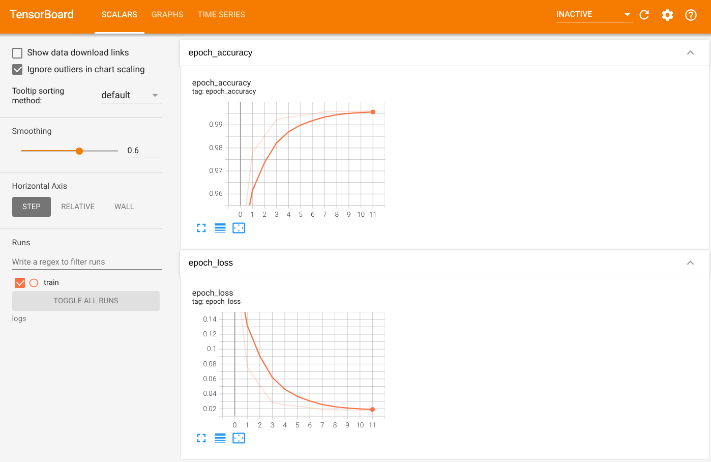
Pour visualiser le résultat, lancez TensorBoard et affichez les journaux :
%tensorboard --logdir=logs
ls -sh ./logs
total 4.0K
4.0K train
Exporter vers le modèle enregistré
Exportez le graphique et les variables au format SavedModel indépendant de la plate-forme à l'aide Model.save . Une fois votre modèle enregistré, vous pouvez le charger avec ou sans Strategy.scope .
path = 'saved_model/'
model.save(path, save_format='tf')
2022-01-26 05:39:18.012847: W tensorflow/python/util/util.cc:368] Sets are not currently considered sequences, but this may change in the future, so consider avoiding using them.
INFO:tensorflow:Assets written to: saved_model/assets
INFO:tensorflow:Assets written to: saved_model/assets
Maintenant, chargez le modèle sans Strategy.scope :
unreplicated_model = tf.keras.models.load_model(path)

unreplicated_model.compile(
    loss=tf.keras.losses.SparseCategoricalCrossentropy(from_logits=True),
    optimizer=tf.keras.optimizers.Adam(),
    metrics=['accuracy'])

eval_loss, eval_acc = unreplicated_model.evaluate(eval_dataset)

print('Eval loss: {}, Eval Accuracy: {}'.format(eval_loss, eval_acc))
157/157 [==============================] - 1s 2ms/step - loss: 0.0373 - accuracy: 0.9879
Eval loss: 0.03732967749238014, Eval Accuracy: 0.9879000186920166
Chargez le modèle avec Strategy.scope :
with strategy.scope():
  replicated_model = tf.keras.models.load_model(path)
  replicated_model.compile(loss=tf.keras.losses.SparseCategoricalCrossentropy(from_logits=True),
                           optimizer=tf.keras.optimizers.Adam(),
                           metrics=['accuracy'])

  eval_loss, eval_acc = replicated_model.evaluate(eval_dataset)
  print ('Eval loss: {}, Eval Accuracy: {}'.format(eval_loss, eval_acc))
2022-01-26 05:39:19.489971: W tensorflow/core/grappler/optimizers/data/auto_shard.cc:547] The `assert_cardinality` transformation is currently not handled by the auto-shard rewrite and will be removed.
157/157 [==============================] - 3s 3ms/step - loss: 0.0373 - accuracy: 0.9879
Eval loss: 0.03732967749238014, Eval Accuracy: 0.9879000186920166
Ressources additionnelles
Autres exemples utilisant différentes stratégies de distribution avec l'API Keras Model.fit :
- Le didacticiel Résoudre les tâches GLUE à l'aide de BERT sur TPU utilise
tf.distribute.MirroredStrategypour la formation sur les GPU ettf.distribute.TPUStrategysur les TPU. - Le didacticiel Enregistrer et charger un modèle à l'aide d'une stratégie de distribution montre comment utiliser les API SavedModel avec
tf.distribute.Strategy. - Les modèles officiels de TensorFlow peuvent être configurés pour exécuter plusieurs stratégies de distribution.
Pour en savoir plus sur les stratégies de distribution TensorFlow :
- Le didacticiel Formation personnalisée avec tf.distribute.Strategy montre comment utiliser
tf.distribute.MirroredStrategypour la formation d'un seul travailleur avec une boucle de formation personnalisée. - Le didacticiel Formation multi-travailleurs avec Keras montre comment utiliser
MultiWorkerMirroredStrategyavecModel.fit. - Le didacticiel Boucle de formation personnalisée avec Keras et MultiWorkerMirroredStrategy montre comment utiliser
MultiWorkerMirroredStrategyavec Keras et une boucle de formation personnalisée. - Le guide Formation distribuée dans TensorFlow fournit une vue d'ensemble des stratégies de distribution disponibles.
- Le guide Meilleures performances avec tf.function fournit des informations sur d'autres stratégies et outils, tels que le profileur TensorFlow , que vous pouvez utiliser pour optimiser les performances de vos modèles TensorFlow.