
 GitHub에서 소스 보기 GitHub에서 소스 보기 |
이 튜토리얼은 TensorFlow에서 CSV 데이터를 사용하는 방법에 대한 예제를 제공합니다.
다음과 같이 두 가지 주요 내용이 있습니다.
- Loading the data off disk
- Pre-processing it into a form suitable for training.
이 튜토리얼은 로딩에 중점을 두며 전처리에 대한 몇 가지 빠른 예를 제공합니다. 전처리 측면에 대해 자세히 알아보려면 전처리 레이어 작업 가이드 및 Keras 전처리 레이어를 사용하여 구조화된 데이터 분류 튜토리얼을 확인하세요.
설정하기
import pandas as pd
import numpy as np

# Make numpy values easier to read.
np.set_printoptions(precision=3, suppress=True)

import tensorflow as tf
from tensorflow.keras import layers
2022-12-14 21:07:04.071551: W tensorflow/compiler/xla/stream_executor/platform/default/dso_loader.cc:64] Could not load dynamic library 'libnvinfer.so.7'; dlerror: libnvinfer.so.7: cannot open shared object file: No such file or directory
2022-12-14 21:07:04.071675: W tensorflow/compiler/xla/stream_executor/platform/default/dso_loader.cc:64] Could not load dynamic library 'libnvinfer_plugin.so.7'; dlerror: libnvinfer_plugin.so.7: cannot open shared object file: No such file or directory
2022-12-14 21:07:04.071686: W tensorflow/compiler/tf2tensorrt/utils/py_utils.cc:38] TF-TRT Warning: Cannot dlopen some TensorRT libraries. If you would like to use Nvidia GPU with TensorRT, please make sure the missing libraries mentioned above are installed properly.
인메모리 데이터
작은 크기의 CSV 데이터세트를 사용하여 TensorFlow 모델을 훈련시키는 가장 간단한 방법은 이를 메모리에 pandas Dataframe 또는 NumPy 배열로 로드하는 것입니다.
비교적 간단한 예는 전복 데이터세트입니다.
- 데이터세트의 크기가 작습니다.
- 모든 입력 특성은 모두 제한된 범위의 부동 소수점 값입니다.
다음은 Pandas DataFrame에 데이터를 다운로드하는 방법입니다.
abalone_train = pd.read_csv(
    "https://storage.googleapis.com/download.tensorflow.org/data/abalone_train.csv",
    names=["Length", "Diameter", "Height", "Whole weight", "Shucked weight",
           "Viscera weight", "Shell weight", "Age"])

abalone_train.head()
이 데이터세트에는 바다 고등류의 일종인 전복 측정값 세트가 포함되어 있습니다.
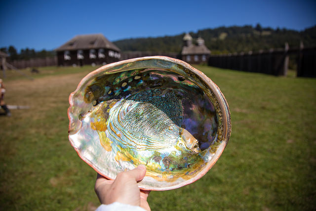
“전복 껍질” (Nicki Dugan Pogue 제공, CC BY-SA 2.0)
이 데이터 세트의 명목상 작업은 다른 측정값으로부터 나이를 예측하는 것이므로 다음과 같이 훈련을 위해 특성과 레이블을 분리합니다.
abalone_features = abalone_train.copy()
abalone_labels = abalone_features.pop('Age')
이 데이터세트에서는 모든 특성을 동일하게 취급합니다. 다음과 같이 특성을 단일 NumPy 배열로 묶습니다.
abalone_features = np.array(abalone_features)
abalone_features
array([[0.435, 0.335, 0.11 , ..., 0.136, 0.077, 0.097],
       [0.585, 0.45 , 0.125, ..., 0.354, 0.207, 0.225],
       [0.655, 0.51 , 0.16 , ..., 0.396, 0.282, 0.37 ],
       ...,
       [0.53 , 0.42 , 0.13 , ..., 0.374, 0.167, 0.249],
       [0.395, 0.315, 0.105, ..., 0.118, 0.091, 0.119],
       [0.45 , 0.355, 0.12 , ..., 0.115, 0.067, 0.16 ]])
다음으로, 회귀 모델로 나이를 예측합니다. 입력 텐서가 하나만 있으므로 여기에서는 keras.Sequential 모델이면 충분합니다.
abalone_model = tf.keras.Sequential([
  layers.Dense(64),
  layers.Dense(1)
])

abalone_model.compile(loss = tf.keras.losses.MeanSquaredError(),
                      optimizer = tf.keras.optimizers.Adam())
해당 모델을 훈련하려면 특성과 레이블을 Model.fit로 전달합니다.
abalone_model.fit(abalone_features, abalone_labels, epochs=10)
Epoch 1/10
104/104 [==============================] - 2s 2ms/step - loss: 73.6423
Epoch 2/10
104/104 [==============================] - 0s 2ms/step - loss: 13.6555
Epoch 3/10
104/104 [==============================] - 0s 2ms/step - loss: 8.5453
Epoch 4/10
104/104 [==============================] - 0s 2ms/step - loss: 8.0819
Epoch 5/10
104/104 [==============================] - 0s 2ms/step - loss: 7.6597
Epoch 6/10
104/104 [==============================] - 0s 2ms/step - loss: 7.3031
Epoch 7/10
104/104 [==============================] - 0s 2ms/step - loss: 7.0281
Epoch 8/10
104/104 [==============================] - 0s 2ms/step - loss: 6.8179
Epoch 9/10
104/104 [==============================] - 0s 2ms/step - loss: 6.6587
Epoch 10/10
104/104 [==============================] - 0s 2ms/step - loss: 6.5618
<keras.callbacks.History at 0x7f4a91c7d580>
지금까지 CSV 데이터를 사용하여 모델을 훈련하는 가장 기본적인 방법을 보았습니다. 다음으로 숫자 열을 정규화하기 위해 전처리를 적용하는 방법을 배웁니다.
기본 전처리
모델에 대한 입력을 정규화하면 좋습니다. Keras 전처리 레이어는 이 정규화를 모델에 빌드하는 편리한 방법을 제공합니다.
tf.keras.layers.Normalization 레이어는 각 열의 평균과 분산을 미리 계산하고 이를 사용하여 데이터를 정규화합니다.
먼저 레이어를 만듭니다.
normalize = layers.Normalization()
그런 다음 Normalization.adapt 메서드를 사용하여 정규화 레이어를 데이터에 맞게 조정합니다.
참고: PreprocessingLayer.adapt 메서드와 함께 훈련 데이터만 사용하고 검증 또는 테스트 데이터는 사용하지 마세요.
normalize.adapt(abalone_features)
그런 다음 모델에서 정규화 레이어를 사용합니다.
norm_abalone_model = tf.keras.Sequential([
  normalize,
  layers.Dense(64),
  layers.Dense(1)
])

norm_abalone_model.compile(loss = tf.keras.losses.MeanSquaredError(),
                           optimizer = tf.keras.optimizers.Adam())

norm_abalone_model.fit(abalone_features, abalone_labels, epochs=10)
Epoch 1/10
104/104 [==============================] - 1s 2ms/step - loss: 92.5604
Epoch 2/10
104/104 [==============================] - 0s 2ms/step - loss: 53.8474
Epoch 3/10
104/104 [==============================] - 0s 2ms/step - loss: 17.0539
Epoch 4/10
104/104 [==============================] - 0s 2ms/step - loss: 5.9795
Epoch 5/10
104/104 [==============================] - 0s 2ms/step - loss: 5.0962
Epoch 6/10
104/104 [==============================] - 0s 2ms/step - loss: 5.0296
Epoch 7/10
104/104 [==============================] - 0s 2ms/step - loss: 4.9844
Epoch 8/10
104/104 [==============================] - 0s 2ms/step - loss: 4.9694
Epoch 9/10
104/104 [==============================] - 0s 2ms/step - loss: 4.9474
Epoch 10/10
104/104 [==============================] - 0s 2ms/step - loss: 4.9429
<keras.callbacks.History at 0x7f4a6c4b62e0>
혼합 데이터 유형
The "Titanic" dataset contains information about the passengers on the Titanic. The nominal task on this dataset is to predict who survived.
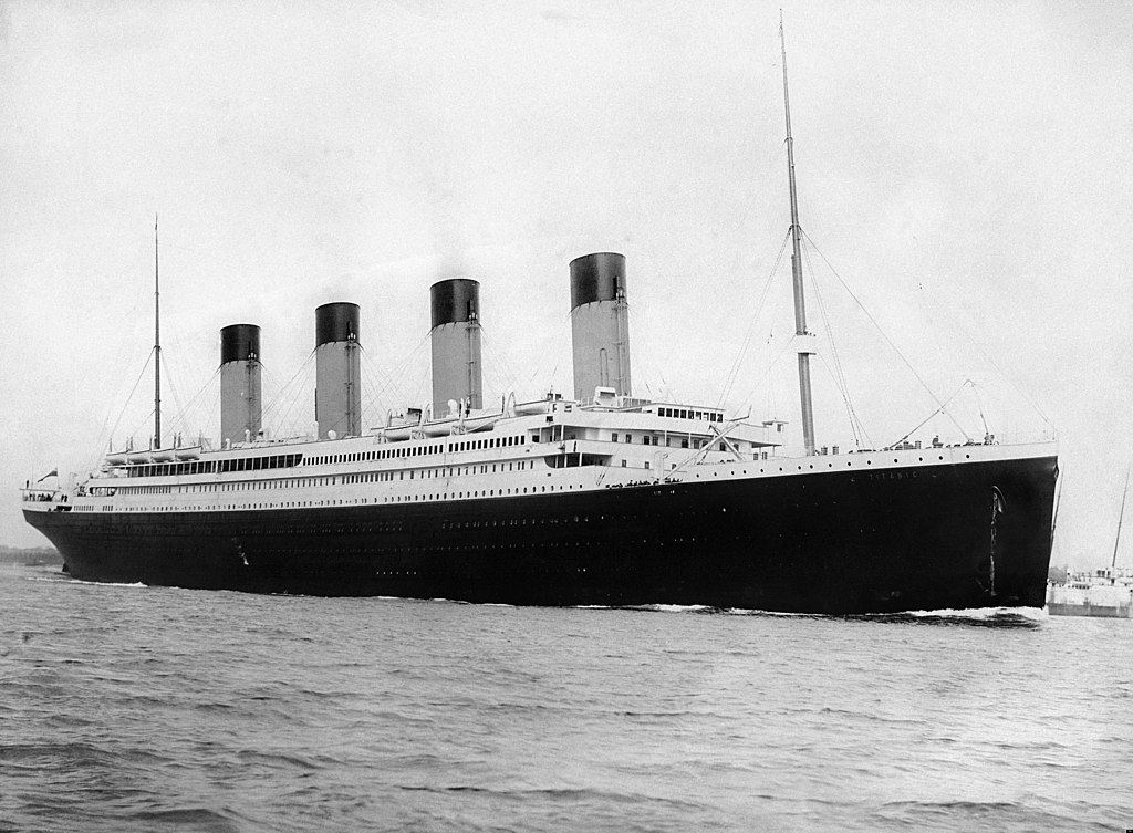
Image from Wikimedia
The raw data can easily be loaded as a Pandas DataFrame, but is not immediately usable as input to a TensorFlow model.
titanic = pd.read_csv("https://storage.googleapis.com/tf-datasets/titanic/train.csv")
titanic.head()
titanic_features = titanic.copy()
titanic_labels = titanic_features.pop('survived')
데이터 유형과 범위가 다르기 때문에 단순히 특성을 NumPy 배열에 쌓아서 keras.Sequential 모델로 전달할 수 없습니다. 각 열을 개별적으로 처리해야 합니다.
한 가지 옵션으로 데이터를 오프라인으로 전처리(원하는 도구 사용)하여 범주형 열을 숫자 열로 변환한 다음 처리된 출력을 TensorFlow 모델에 전달할 수 있습니다. 이 접근 방식의 단점은 모델을 저장하고 내보내는 경우 전처리가 함께 저장되지 않는다는 것입니다. Keras 전처리 레이어는 모델의 일부이기 때문에 이 문제를 피할 수 있습니다.
이 예제에서는 Keras 함수형 API를 사용하여 전처리 로직을 구현하는 모델을 빌드합니다. 하위 클래스화하여 같은 작업을 수행할 수도 있습니다.
함수형 API는 "기호화된" 텐서에서 작동합니다. 정상적인 "즉시(eager)" 텐서에는 값이 있습니다. 대조적으로 이러한 "기호화된" 텐서에는 값이 없습니다. 대신에 실행되는 작업을 추적하고 나중에 실행할 수 있는 계산 표현을 작성합니다. 다음은 간단한 예제입니다.
# Create a symbolic input
input = tf.keras.Input(shape=(), dtype=tf.float32)

# Perform a calculation using the input
result = 2*input + 1

# the result doesn't have a value
result
<KerasTensor: shape=(None,) dtype=float32 (created by layer 'tf.__operators__.add')>
calc = tf.keras.Model(inputs=input, outputs=result)
print(calc(1).numpy())
print(calc(2).numpy())
3.0
5.0
전처리 모델을 빌드하려면 먼저 CSV 열의 이름 및 데이터 유형과 일치하는 기호화된 tf.keras.Input 객체 세트를 빌드합니다.
inputs = {}

for name, column in titanic_features.items():
  dtype = column.dtype
  if dtype == object:
    dtype = tf.string
  else:
    dtype = tf.float32

  inputs[name] = tf.keras.Input(shape=(1,), name=name, dtype=dtype)

inputs
{'sex': <KerasTensor: shape=(None, 1) dtype=string (created by layer 'sex')>,
 'age': <KerasTensor: shape=(None, 1) dtype=float32 (created by layer 'age')>,
 'n_siblings_spouses': <KerasTensor: shape=(None, 1) dtype=float32 (created by layer 'n_siblings_spouses')>,
 'parch': <KerasTensor: shape=(None, 1) dtype=float32 (created by layer 'parch')>,
 'fare': <KerasTensor: shape=(None, 1) dtype=float32 (created by layer 'fare')>,
 'class': <KerasTensor: shape=(None, 1) dtype=string (created by layer 'class')>,
 'deck': <KerasTensor: shape=(None, 1) dtype=string (created by layer 'deck')>,
 'embark_town': <KerasTensor: shape=(None, 1) dtype=string (created by layer 'embark_town')>,
 'alone': <KerasTensor: shape=(None, 1) dtype=string (created by layer 'alone')>}
전처리 논리의 첫 번째 단계는 숫자 입력을 함께 연결하고 이를 정규화 레이어를 통해 실행하는 것입니다.
numeric_inputs = {name:input for name,input in inputs.items()
                  if input.dtype==tf.float32}

x = layers.Concatenate()(list(numeric_inputs.values()))
norm = layers.Normalization()
norm.adapt(np.array(titanic[numeric_inputs.keys()]))
all_numeric_inputs = norm(x)

all_numeric_inputs
<KerasTensor: shape=(None, 4) dtype=float32 (created by layer 'normalization_1')>
나중에 연결할 수 있도록 모든 기호화된 전처리 결과를 수집합니다.
preprocessed_inputs = [all_numeric_inputs]
문자열 입력의 경우 tf.keras.layers.StringLookup 함수를 사용하여 문자열로부터 어휘의 정수 인덱스로 매핑합니다. 그런 다음 tf.keras.layers.CategoryEncoding을 사용하여 인덱스를 모델에 적합한 float32 데이터로 변환합니다.
tf.keras.layers.CategoryEncoding 레이어의 기본 설정은 각 입력에 대해 원-핫 벡터를 생성하는 것입니다. tf.keras.layers.Embedding도 작동합니다. 이 주제에 대한 자세한 내용은 전처리 레이어 작업 가이드 및 Keras 전처리 레이어를 사용하여 구조화된 데이터 분류 튜토리얼을 확인하세요.
for name, input in inputs.items():
  if input.dtype == tf.float32:
    continue

  lookup = layers.StringLookup(vocabulary=np.unique(titanic_features[name]))
  one_hot = layers.CategoryEncoding(num_tokens=lookup.vocabulary_size())

  x = lookup(input)
  x = one_hot(x)
  preprocessed_inputs.append(x)
inputs 및 preprocessed_inputs 모음을 사용하여 전처리된 모든 입력을 함께 연결하고 전처리를 처리하는 모델을 빌드할 수 있습니다.
preprocessed_inputs_cat = layers.Concatenate()(preprocessed_inputs)

titanic_preprocessing = tf.keras.Model(inputs, preprocessed_inputs_cat)

tf.keras.utils.plot_model(model = titanic_preprocessing , rankdir="LR", dpi=72, show_shapes=True)
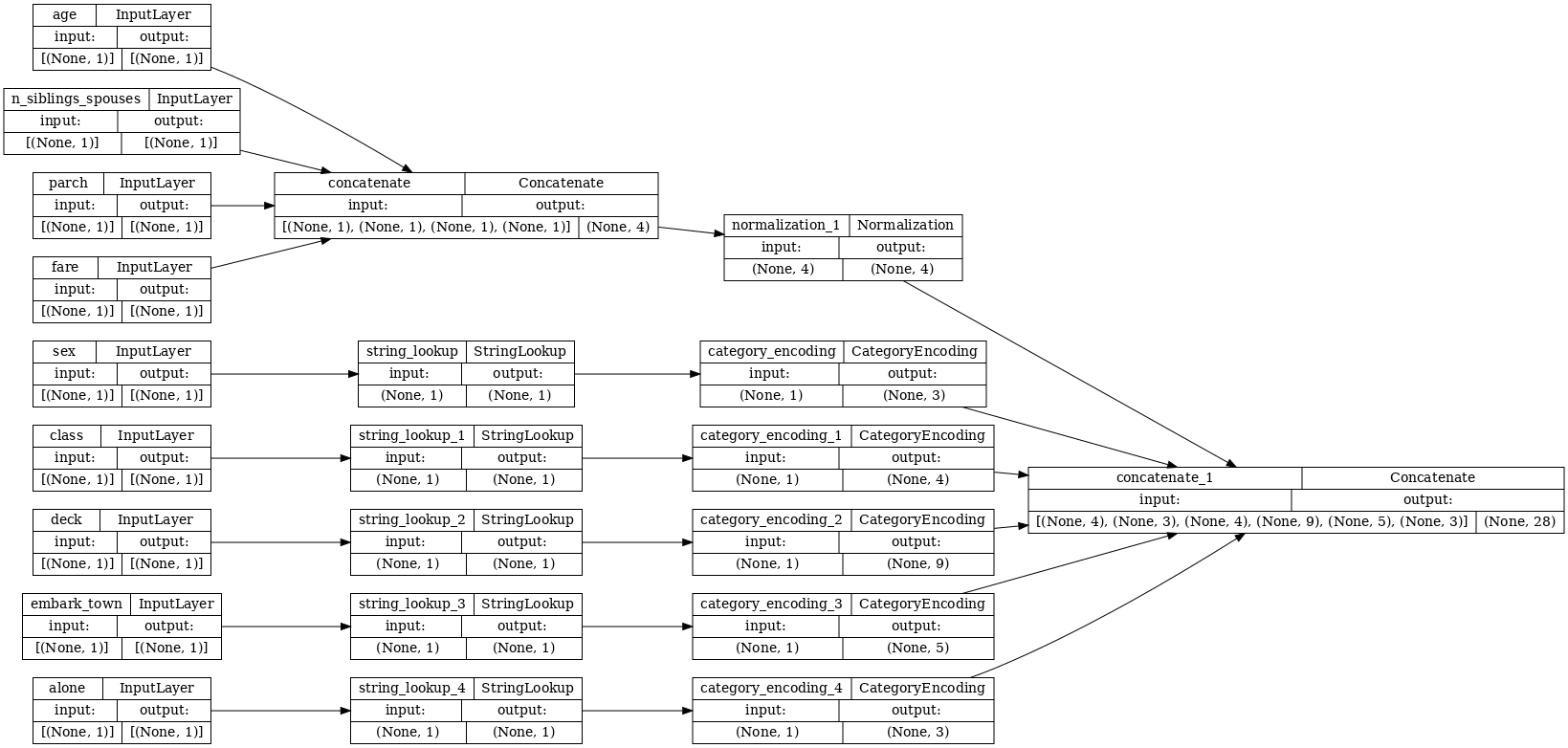
이 모델은 입력 전처리만 포함합니다. 이를 실행하여 데이터에 어떤 영향을 미치는지 확인할 수 있습니다. Keras 모델은 Pandas DataFrames를 자동으로 변환하지 않습니다. 왜냐하면 하나의 텐서로 변환해야 하는지 아니면 텐서 사전으로 변환해야 하는지가 명확하지 않기 때문입니다. 따라서 이를 텐서 사전으로 변환합니다.
titanic_features_dict = {name: np.array(value)
                         for name, value in titanic_features.items()}
첫 번째 훈련 예제를 잘라서 이 전처리 모델로 전달하면 숫자 특성과 문자열 원-핫이 모두 함께 연결된 것을 볼 수 있습니다.
features_dict = {name:values[:1] for name, values in titanic_features_dict.items()}
titanic_preprocessing(features_dict)
<tf.Tensor: shape=(1, 28), dtype=float32, numpy=
array([[-0.61 ,  0.395, -0.479, -0.497,  0.   ,  0.   ,  1.   ,  0.   ,

         0.   ,  0.   ,  1.   ,  0.   ,  0.   ,  0.   ,  0.   ,  0.   ,
         0.   ,  0.   ,  0.   ,  1.   ,  0.   ,  0.   ,  0.   ,  1.   ,
         0.   ,  0.   ,  1.   ,  0.   ]], dtype=float32)>
이제 이 위에 모델을 빌드합니다.
def titanic_model(preprocessing_head, inputs):
  body = tf.keras.Sequential([
    layers.Dense(64),
    layers.Dense(1)
  ])

  preprocessed_inputs = preprocessing_head(inputs)
  result = body(preprocessed_inputs)
  model = tf.keras.Model(inputs, result)

  model.compile(loss=tf.keras.losses.BinaryCrossentropy(from_logits=True),
                optimizer=tf.keras.optimizers.Adam())
  return model

titanic_model = titanic_model(titanic_preprocessing, inputs)
모델을 훈련할 때 특성 사전을 x로, 레이블을 y로 전달합니다.
titanic_model.fit(x=titanic_features_dict, y=titanic_labels, epochs=10)
Epoch 1/10
20/20 [==============================] - 1s 5ms/step - loss: 0.5686
Epoch 2/10
20/20 [==============================] - 0s 4ms/step - loss: 0.5040
Epoch 3/10
20/20 [==============================] - 0s 4ms/step - loss: 0.4742
Epoch 4/10
20/20 [==============================] - 0s 4ms/step - loss: 0.4549
Epoch 5/10
20/20 [==============================] - 0s 4ms/step - loss: 0.4436
Epoch 6/10
20/20 [==============================] - 0s 4ms/step - loss: 0.4349
Epoch 7/10
20/20 [==============================] - 0s 4ms/step - loss: 0.4297
Epoch 8/10
20/20 [==============================] - 0s 4ms/step - loss: 0.4266
Epoch 9/10
20/20 [==============================] - 0s 4ms/step - loss: 0.4252
Epoch 10/10
20/20 [==============================] - 0s 4ms/step - loss: 0.4230
<keras.callbacks.History at 0x7f4b77aa7a60>
전처리는 모델의 일부이므로 모델을 저장하고 다른 곳에 다시 로드하여도 동일한 결과를 얻을 수 있습니다.
titanic_model.save('test')
reloaded = tf.keras.models.load_model('test')
INFO:tensorflow:Assets written to: test/assets
features_dict = {name:values[:1] for name, values in titanic_features_dict.items()}

before = titanic_model(features_dict)
after = reloaded(features_dict)
assert (before-after)<1e-3
print(before)
print(after)
tf.Tensor([[-1.923]], shape=(1, 1), dtype=float32)
tf.Tensor([[-1.923]], shape=(1, 1), dtype=float32)
tf.data 사용하기
이전 섹션에서는 모델을 훈련하는 동안 모델의 내장 데이터 셔플링 및 배치에 의존했습니다.
입력 데이터 파이프라인을 더 많이 제어해야 하거나 메모리에 쉽게 맞출 수 없는 데이터를 사용해야 하는 경우 tf.data를 사용합니다.
더 많은 예를 보려면 tf.data: TensorFlow 입력 파이프라인 빌드 가이드를 참조하세요.
인메모리 데이터에서
CSV 데이터에 tf.data를 적용하는 첫 번째 예제로 다음 코드를 고려할 경우 이전 섹션의 특성 사전을 수동으로 분할합니다. 각 인덱스에는 각 특성에 대해 이러한 인덱스를 사용합니다.
import itertools

def slices(features):
  for i in itertools.count():
    # For each feature take index `i`
    example = {name:values[i] for name, values in features.items()}
    yield example
이것을 실행하고 첫 번째 예제를 출력합니다.
for example in slices(titanic_features_dict):
  for name, value in example.items():
    print(f"{name:19s}: {value}")
  break
sex                : male
age                : 22.0
n_siblings_spouses : 1
parch              : 0
fare               : 7.25
class              : Third
deck               : unknown
embark_town        : Southampton
alone              : n
메모리 데이터 로더에서 가장 기본적인 tf.data.Dataset은 Dataset.from_tensor_slices 생성자입니다. 이것은 TensorFlow에서 위의 slices 함수의 일반화된 버전을 구현하는 tf.data.Dataset를 반환합니다.
features_ds = tf.data.Dataset.from_tensor_slices(titanic_features_dict)
다른 Python iterable과 마찬가지로 tf.data.Dataset에 대해 반복할 수 있습니다.
for example in features_ds:
  for name, value in example.items():
    print(f"{name:19s}: {value}")
  break
sex                : b'male'
age                : 22.0
n_siblings_spouses : 1
parch              : 0
fare               : 7.25
class              : b'Third'
deck               : b'unknown'
embark_town        : b'Southampton'
alone              : b'n'
from_tensor_slices 함수는 모든 구조의 중첩된 사전 또는 튜플을 처리할 수 있습니다. 다음 코드는 (features_dict, labels) 쌍의 데이터세트를 만듭니다.
titanic_ds = tf.data.Dataset.from_tensor_slices((titanic_features_dict, titanic_labels))
이 Dataset를 사용하여 모델을 훈련하려면 최소한 데이터를 shuffle하고 batch 처리해야 합니다.
titanic_batches = titanic_ds.shuffle(len(titanic_labels)).batch(32)
features 및 labels를 Model.fit에 전달하는 대신 데이터세트를 전달합니다.
titanic_model.fit(titanic_batches, epochs=5)
Epoch 1/5
20/20 [==============================] - 1s 4ms/step - loss: 0.4216
Epoch 2/5
20/20 [==============================] - 0s 4ms/step - loss: 0.4205
Epoch 3/5
20/20 [==============================] - 0s 4ms/step - loss: 0.4214
Epoch 4/5
20/20 [==============================] - 0s 4ms/step - loss: 0.4193
Epoch 5/5
20/20 [==============================] - 0s 4ms/step - loss: 0.4196
<keras.callbacks.History at 0x7f4a92453e80>
단일 파일로부터
지금까지 이 튜토리얼은 인메모리 데이터로 작업했습니다. tf.data는 데이터 파이프라인을 빌드하기 위한 확장성이 뛰어난 툴킷이며 CSV 파일 로드를 처리하는 몇 가지 기능을 제공합니다.
titanic_file_path = tf.keras.utils.get_file("train.csv", "https://storage.googleapis.com/tf-datasets/titanic/train.csv")
Downloading data from https://storage.googleapis.com/tf-datasets/titanic/train.csv
30874/30874 [==============================] - 0s 0us/step
이제 파일에서 CSV 데이터를 읽고 tf.data.Dataset를 작성합니다.
(전체 설명서는 tf.data.experimental.make_csv_dataset를 참조하세요.)
titanic_csv_ds = tf.data.experimental.make_csv_dataset(
    titanic_file_path,
    batch_size=5, # Artificially small to make examples easier to show.
    label_name='survived',
    num_epochs=1,
    ignore_errors=True,)
WARNING:tensorflow:From /tmpfs/src/tf_docs_env/lib/python3.9/site-packages/tensorflow/python/data/experimental/ops/readers.py:572: ignore_errors (from tensorflow.python.data.experimental.ops.error_ops) is deprecated and will be removed in a future version.
Instructions for updating:
Use `tf.data.Dataset.ignore_errors` instead.
이 함수에는 많은 편리한 특성이 포함되어 있어 데이터 작업이 용이합니다. 여기에는 다음이 포함되어 있습니다.
- 열 헤더를 사전 키로 사용.
- 각 열의 유형을 자동으로 결정.
주의: tf.data.experimental.make_csv_dataset에서 num_epochs 인수를 설정해야 합니다. 그렇지 않으면 tf.data.Dataset의 기본 동작은 루프를 무한히 반복하는 것입니다.
for batch, label in titanic_csv_ds.take(1):
  for key, value in batch.items():
    print(f"{key:20s}: {value}")
  print()
  print(f"{'label':20s}: {label}")
sex                 : [b'male' b'female' b'male' b'female' b'male']
age                 : [26. 42. 32. 21. 46.]
n_siblings_spouses  : [0 0 0 0 0]
parch               : [0 0 0 0 0]
fare                : [ 8.05 13.    8.05  7.75 79.2 ]
class               : [b'Third' b'Second' b'Third' b'Third' b'First']
deck                : [b'unknown' b'unknown' b'E' b'unknown' b'B']
embark_town         : [b'Southampton' b'Southampton' b'Southampton' b'Queenstown' b'Cherbourg']
alone               : [b'y' b'y' b'y' b'y' b'y']

label               : [0 1 1 0 0]
참고: 위의 셀을 두 번 실행하면 다른 결과가 생성됩니다. tf.data.experimental.make_csv_dataset의 기본 설정에는 shuffle_buffer_size=1000이 포함되며, 이는 이 작은 데이터세트에는 충분하지만 실제 데이터세트에는 그렇지 않을 수 있습니다.
즉시 데이터 압축을 풀 수도 있습니다. 다음은 대도시 주간 교통량 데이터세트가 포함된 gzip으로 압축된 CSV 파일입니다.
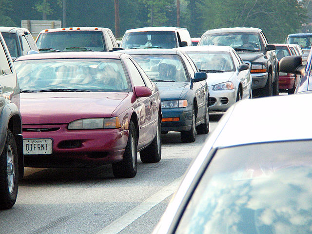
이미지 출처: Wikimedia
traffic_volume_csv_gz = tf.keras.utils.get_file(
    'Metro_Interstate_Traffic_Volume.csv.gz',
    "https://archive.ics.uci.edu/ml/machine-learning-databases/00492/Metro_Interstate_Traffic_Volume.csv.gz",
    cache_dir='.', cache_subdir='traffic')
Downloading data from https://archive.ics.uci.edu/ml/machine-learning-databases/00492/Metro_Interstate_Traffic_Volume.csv.gz
405373/405373 [==============================] - 0s 0us/step
압축된 파일로부터 직접 읽도록 compression_type 인수를 설정합니다.
traffic_volume_csv_gz_ds = tf.data.experimental.make_csv_dataset(
    traffic_volume_csv_gz,
    batch_size=256,
    label_name='traffic_volume',
    num_epochs=1,
    compression_type="GZIP")

for batch, label in traffic_volume_csv_gz_ds.take(1):
  for key, value in batch.items():
    print(f"{key:20s}: {value[:5]}")
  print()
  print(f"{'label':20s}: {label[:5]}")
holiday             : [b'None' b'None' b'None' b'None' b'None']
temp                : [267.84 285.35 266.41 280.66 279.53]
rain_1h             : [0. 0. 0. 0. 0.]
snow_1h             : [0. 0. 0. 0. 0.]
clouds_all          : [90 32 90 90  1]
weather_main        : [b'Snow' b'Clouds' b'Snow' b'Mist' b'Clear']
weather_description : [b'heavy snow' b'scattered clouds' b'heavy snow' b'mist' b'sky is clear']
date_time           : [b'2013-03-19 12:00:00' b'2013-07-29 02:00:00' b'2013-01-03 22:00:00'
 b'2013-05-23 07:00:00' b'2013-04-04 15:00:00']

label               : [4755  324 1550 6717 5992]
참고: tf.data 파이프라인에서 해당 날짜-시간 문자열을 파싱해야 하는 경우 tfa.text.parse_time을 사용할 수 있습니다.
캐싱
CSV 데이터를 파싱하는 데 약간의 오버헤드가 있습니다. 작은 크기의 모델의 경우 이때 훈련 병목 현상이 발생할 수 있습니다.
사용 사례에 따라 CSV 데이터가 첫 번째 epoch에서만 파싱되도록 Dataset.cache 또는 tf.data.experimental.snapshot을 사용하는 것이 좋습니다.
cache와 snapshot 메서드의 주요 차이점은 cache 파일은 이를 생성한 TensorFlow 프로세스에서만 사용할 수 있다는 것입니다. 다만, snapshot 파일은 다른 프로세스에서 읽을 수 있습니다.
예를 들어, traffic_volume_csv_gz_ds를 20번 반복하는 데 캐싱 없이는 약 15초, 캐싱이 있으면 약 2초가 걸릴 수 있습니다.
%%time
for i, (batch, label) in enumerate(traffic_volume_csv_gz_ds.repeat(20)):
  if i % 40 == 0:
    print('.', end='')
print()
...............................................................................................
CPU times: user 17.7 s, sys: 3.98 s, total: 21.6 s
Wall time: 13 s
참고: Dataset.cache는 첫 번째 epoch의 데이터를 저장하고 순서대로 재생합니다. 따라서 cache 메서드를 사용하면 파이프라인의 초기에 모든 셔플이 비활성화됩니다. 아래에서 Dataset.shuffle은 Dataset.cache 뒤에 다시 추가됩니다.
%%time
caching = traffic_volume_csv_gz_ds.cache().shuffle(1000)

for i, (batch, label) in enumerate(caching.shuffle(1000).repeat(20)):
  if i % 40 == 0:
    print('.', end='')
print()
...............................................................................................
CPU times: user 1.98 s, sys: 293 ms, total: 2.27 s
Wall time: 1.78 s
참고: tf.data.experimental.snapshot 파일은 사용 중 데이터세트를 임시로 저장하기 위한 것입니다. 이것은 장기 보관을 위한 형식이 아닙니다. 파일 형식은 내부 정보로 간주되며 TensorFlow 버전 간에 보장되지 않습니다.
%%time
snapshot = tf.data.experimental.snapshot('titanic.tfsnap')
snapshotting = traffic_volume_csv_gz_ds.apply(snapshot).shuffle(1000)

for i, (batch, label) in enumerate(snapshotting.shuffle(1000).repeat(20)):
  if i % 40 == 0:
    print('.', end='')
print()
WARNING:tensorflow:From <timed exec>:1: snapshot (from tensorflow.python.data.experimental.ops.snapshot) is deprecated and will be removed in a future version.
Instructions for updating:
Use `tf.data.Dataset.snapshot(...)`.
...............................................................................................
CPU times: user 3.03 s, sys: 814 ms, total: 3.84 s
Wall time: 2.06 s
CSV 파일 로드로 인해 데이터 로드가 느려지고 Dataset.cache 및 tf.data.experimental.snapshot이 사용 사례에 충분하지 않은 경우, 데이터를 보다 간소화된 형식으로 다시 인코딩하는 것이 좋습니다.
여러 파일
지금까지 이 섹션의 모든 예제는 tf.data 없이 쉽게 수행할 수 있었습니다. tf.data를 사용하여 실제로 작업을 단순화할 수 있는 한 예는 파일 모음을 처리할 경우입니다.
예를 들어 문자 글꼴 이미지 데이터세트는 글꼴당 하나씩, csv 파일 모음으로 배포됩니다.
Pixabay에서 Willi Heidelbach가 제공한 이미지
데이터세트를 다운로드하고 내부 파일을 검토합니다.
fonts_zip = tf.keras.utils.get_file(
    'fonts.zip',  "https://archive.ics.uci.edu/ml/machine-learning-databases/00417/fonts.zip",
    cache_dir='.', cache_subdir='fonts',
    extract=True)
Downloading data from https://archive.ics.uci.edu/ml/machine-learning-databases/00417/fonts.zip
160313983/160313983 [==============================] - 3s 0us/step
import pathlib
font_csvs =  sorted(str(p) for p in pathlib.Path('fonts').glob("*.csv"))

font_csvs[:10]
['fonts/AGENCY.csv',
 'fonts/ARIAL.csv',
 'fonts/BAITI.csv',
 'fonts/BANKGOTHIC.csv',
 'fonts/BASKERVILLE.csv',
 'fonts/BAUHAUS.csv',
 'fonts/BELL.csv',
 'fonts/BERLIN.csv',
 'fonts/BERNARD.csv',
 'fonts/BITSTREAMVERA.csv']
len(font_csvs)
153
많은 파일을 처리할 경우 glob 스타일의 file_pattern을 tf.data.experimental.make_csv_dataset 함수에 전달할 수 있습니다. 파일의 순서는 각 반복마다 뒤섞입니다.
num_parallel_reads 인수를 사용하여 병렬로 읽고 함께 인터리브 처리되는 파일의 수를 설정합니다.
fonts_ds = tf.data.experimental.make_csv_dataset(
    file_pattern = "fonts/*.csv",
    batch_size=10, num_epochs=1,
    num_parallel_reads=20,
    shuffle_buffer_size=10000)
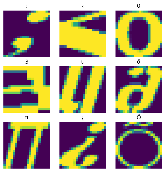
이러한 CSV 파일의 이미지는 단일 행으로 평면화되어 있습니다. 열 이름의 형식은 r{row}c{column}입니다. 다음은 첫 번째 배치입니다.
for features in fonts_ds.take(1):
  for i, (name, value) in enumerate(features.items()):
    if i>15:
      break
    print(f"{name:20s}: {value}")
print('...')
print(f"[total: {len(features)} features]")
font                : [b'BOOK' b'BOOK' b'BASKERVILLE' b'BASKERVILLE' b'PANROMAN'
 b'CITYBLUEPRINT' b'MAGNETO' b'HIMALAYA' b'VLADIMIR' b'BOOK']
fontVariant         : [b'BOOK ANTIQUA' b'BOOK ANTIQUA' b'BASKERVILLE OLD FACE'
 b'BASKERVILLE OLD FACE' b'PANROMAN' b'CITYBLUEPRINT' b'MAGNETO'
 b'MICROSOFT HIMALAYA' b'VLADIMIR SCRIPT' b'BOOK ANTIQUA']
m_label             : [ 1045  8211   181   214  8230 61498   180   126    66  8595]
strength            : [0.4 0.4 0.4 0.4 0.4 0.4 0.4 0.4 0.4 0.4]
italic              : [0 0 0 1 0 0 0 0 0 0]
orientation         : [0. 0. 0. 0. 0. 0. 0. 0. 0. 0.]
m_top               : [38 66 48 22 20 60 45 45 33 36]
m_left              : [21 22 19 30 24 26 38 20 25 25]
originalH           : [46  5 44 58 55 31 10  6 49 62]
originalW           : [38 29 32 50 25  2 14 24 58 23]
h                   : [20 20 20 20 20 20 20 20 20 20]
w                   : [20 20 20 20 20 20 20 20 20 20]
r0c0                : [222   1   1   1 255 255   1   1   1   1]
r0c1                : [222 255  32   1 255 255   1   1   1   1]
r0c2                : [234 255 255   1 255 255   1 128   1   1]
r0c3                : [255 255 255   1 255 255   1 255   1   1]
...
[total: 412 features]
선택 사항: 패킹 필드
여러분은 아마도 이와 같이 별도의 열에 있는 각 픽셀로 작업하고 싶지는 않을 것입니다. 이 데이터세트를 사용하기 전에 픽셀을 이미지 텐서로 패킹해야 합니다.
다음은 각 예제의 이미지를 빌드하기 위해 열 이름을 파싱하는 코드입니다.
import re

def make_images(features):
  image = [None]*400
  new_feats = {}

  for name, value in features.items():
    match = re.match('r(\d+)c(\d+)', name)
    if match:
      image[int(match.group(1))*20+int(match.group(2))] = value
    else:
      new_feats[name] = value

  image = tf.stack(image, axis=0)
  image = tf.reshape(image, [20, 20, -1])
  new_feats['image'] = image

  return new_feats
데이터세트의 각 배치에 해당 함수를 적용합니다.
fonts_image_ds = fonts_ds.map(make_images)

for features in fonts_image_ds.take(1):
  break
결과 이미지를 플롯합니다.
from matplotlib import pyplot as plt

plt.figure(figsize=(6,6), dpi=120)

for n in range(9):
  plt.subplot(3,3,n+1)
  plt.imshow(features['image'][..., n])
  plt.title(chr(features['m_label'][n]))
  plt.axis('off')
하위 수준 함수
지금까지 이 튜토리얼은 csv 데이터를 읽기 위한 가장 높은 수준의 유틸리티에 중점을 두었습니다. 사용 사례가 이 기본 패턴에 맞지 않는 경우 고급 사용자에게 도움이 될 수 있는 다른 두 가지 API가 있습니다.
tf.io.decode_csv: 텍스트 줄을 CSV 열 텐서 목록으로 파싱하는 함수입니다.tf.data.experimental.CsvDataset: 하위 수준 CSV 데이터세트 생성자입니다.
이 섹션에서는 tf.data.experimental.make_csv_dataset에서 제공하는 기능을 다시 만들어 이 하위 수준 기능을 사용하는 방법을 보여줍니다.
tf.io.decode_csv
이 함수는 문자열 또는 문자열 목록을 열 목록으로 디코딩합니다.
tf.data.experimental.make_csv_dataset과 달리 이 함수는 열 데이터 유형을 추측하지 않습니다. 각 열에 대해 올바른 유형의 값이 포함된 record_defaults 목록을 제공하여 열 유형을 지정합니다.
tf.io.decode_csv를 사용하여 타이타닉 데이터를 문자열로 읽기 위해 다음과 같이 할 수 있습니다.
text = pathlib.Path(titanic_file_path).read_text()
lines = text.split('\n')[1:-1]

all_strings = [str()]*10
all_strings
['', '', '', '', '', '', '', '', '', '']
features = tf.io.decode_csv(lines, record_defaults=all_strings)

for f in features:
  print(f"type: {f.dtype.name}, shape: {f.shape}")
type: string, shape: (627,)
type: string, shape: (627,)
type: string, shape: (627,)
type: string, shape: (627,)
type: string, shape: (627,)
type: string, shape: (627,)
type: string, shape: (627,)
type: string, shape: (627,)
type: string, shape: (627,)
type: string, shape: (627,)
실제 유형으로 파싱하려면 해당 유형의 record_defaults 목록을 만듭니다.
print(lines[0])
0,male,22.0,1,0,7.25,Third,unknown,Southampton,n
titanic_types = [int(), str(), float(), int(), int(), float(), str(), str(), str(), str()]
titanic_types
[0, '', 0.0, 0, 0, 0.0, '', '', '', '']
features = tf.io.decode_csv(lines, record_defaults=titanic_types)

for f in features:
  print(f"type: {f.dtype.name}, shape: {f.shape}")
type: int32, shape: (627,)
type: string, shape: (627,)
type: float32, shape: (627,)
type: int32, shape: (627,)
type: int32, shape: (627,)
type: float32, shape: (627,)
type: string, shape: (627,)
type: string, shape: (627,)
type: string, shape: (627,)
type: string, shape: (627,)
참고: CSV 텍스트의 개별 라인보다 대형 라인 배치에서 tf.io.decode_csv를 호출하는 것이 더 효율적입니다.
tf.data.experimental.CsvDataset
tf.data.experimental.CsvDataset 클래스는 tf.data.experimental.make_csv_dataset 함수의 편리한 특성인 열 헤더 파싱, 열 유형 추론, 자동 셔플링, 파일 인터리빙 없이 최소한의 CSV Dataset 인터페이스를 제공합니다.
이 생성자는 tf.io.decode_csv와 같은 방식으로 record_defaults를 사용합니다.
simple_titanic = tf.data.experimental.CsvDataset(titanic_file_path, record_defaults=titanic_types, header=True)

for example in simple_titanic.take(1):
  print([e.numpy() for e in example])
[0, b'male', 22.0, 1, 0, 7.25, b'Third', b'unknown', b'Southampton', b'n']
위의 코드는 기본적으로 다음과 같습니다.
def decode_titanic_line(line):
  return tf.io.decode_csv(line, titanic_types)

manual_titanic = (
    # Load the lines of text
    tf.data.TextLineDataset(titanic_file_path)
    # Skip the header row.
    .skip(1)
    # Decode the line.
    .map(decode_titanic_line)
)

for example in manual_titanic.take(1):
  print([e.numpy() for e in example])
[0, b'male', 22.0, 1, 0, 7.25, b'Third', b'unknown', b'Southampton', b'n']
여러 파일
tf.data.experimental.CsvDataset을 사용하여 글꼴 데이터세트를 파싱하려면 먼저 record_defaults에 대한 열 유형을 결정해야 합니다. 우선 한 파일의 첫 번째 행을 검사합니다.
font_line = pathlib.Path(font_csvs[0]).read_text().splitlines()[1]
print(font_line)
AGENCY,AGENCY FB,64258,0.400000,0,0.000000,35,21,51,22,20,20,1,1,1,21,101,210,255,255,255,255,255,255,255,255,255,255,255,255,255,255,1,1,1,93,255,255,255,176,146,146,146,146,146,146,146,146,216,255,255,255,1,1,1,93,255,255,255,70,1,1,1,1,1,1,1,1,163,255,255,255,1,1,1,93,255,255,255,70,1,1,1,1,1,1,1,1,163,255,255,255,1,1,1,93,255,255,255,70,1,1,1,1,1,1,1,1,163,255,255,255,1,1,1,93,255,255,255,70,1,1,1,1,1,1,1,1,163,255,255,255,1,1,1,93,255,255,255,70,1,1,1,1,1,1,1,1,163,255,255,255,141,141,141,182,255,255,255,172,141,141,141,115,1,1,1,1,163,255,255,255,255,255,255,255,255,255,255,255,255,255,255,209,1,1,1,1,163,255,255,255,6,6,6,96,255,255,255,74,6,6,6,5,1,1,1,1,163,255,255,255,1,1,1,93,255,255,255,70,1,1,1,1,1,1,1,1,163,255,255,255,1,1,1,93,255,255,255,70,1,1,1,1,1,1,1,1,163,255,255,255,1,1,1,93,255,255,255,70,1,1,1,1,1,1,1,1,163,255,255,255,1,1,1,93,255,255,255,70,1,1,1,1,1,1,1,1,163,255,255,255,1,1,1,93,255,255,255,70,1,1,1,1,1,1,1,1,163,255,255,255,1,1,1,93,255,255,255,70,1,1,1,1,1,1,1,1,163,255,255,255,1,1,1,93,255,255,255,70,1,1,1,1,1,1,1,1,163,255,255,255,1,1,1,93,255,255,255,70,1,1,1,1,1,1,1,1,163,255,255,255,1,1,1,93,255,255,255,70,1,1,1,1,1,1,1,1,163,255,255,255,1,1,1,93,255,255,255,70,1,1,1,1,1,1,1,1,163,255,255,255
처음 두 개의 필드만 문자열이고 나머지는 정수 또는 부동 소수점이며 쉼표를 계산하여 총 특성 수를 얻을 수 있습니다.
num_font_features = font_line.count(',')+1
font_column_types = [str(), str()] + [float()]*(num_font_features-2)
tf.data.experimental.CsvDataset 생성자는 입력 파일 목록을 가져올 수 있지만 순차적으로 읽습니다. CSV 목록의 첫 번째 파일은 AGENCY.csv입니다.
font_csvs[0]
'fonts/AGENCY.csv'
따라서 파일 목록을 CsvDataset에 전달할 때 AGENCY.csv의 레코드를 먼저 읽습니다.
simple_font_ds = tf.data.experimental.CsvDataset(
    font_csvs,
    record_defaults=font_column_types,
    header=True)
for row in simple_font_ds.take(10):
  print(row[0].numpy())
b'AGENCY'
b'AGENCY'
b'AGENCY'
b'AGENCY'
b'AGENCY'
b'AGENCY'
b'AGENCY'
b'AGENCY'
b'AGENCY'
b'AGENCY'
여러 파일을 인터리브하려면 Dataset.interleave를 사용합니다.
CSV 파일 이름이 포함된 초기 데이터세트는 다음과 같습니다.
font_files = tf.data.Dataset.list_files("fonts/*.csv")
이렇게 하면 각 epoch마다 파일 이름을 셔플합니다.
print('Epoch 1:')
for f in list(font_files)[:5]:
  print("    ", f.numpy())
print('    ...')
print()

print('Epoch 2:')
for f in list(font_files)[:5]:
  print("    ", f.numpy())
print('    ...')
Epoch 1:
     b'fonts/VIN.csv'
     b'fonts/KRISTEN.csv'
     b'fonts/SKETCHFLOW.csv'
     b'fonts/CONSTANTIA.csv'
     b'fonts/PALACE.csv'
    ...

Epoch 2:
     b'fonts/VERDANA.csv'
     b'fonts/SERIF.csv'
     b'fonts/FRENCH.csv'
     b'fonts/MATURA.csv'
     b'fonts/TECHNIC.csv'
    ...
interleave 메서드는 상위 Dataset의 각 요소마다 하위 Dataset를 생성하는 map_func를 사용합니다.
여기에서 파일 데이터세트의 각 요소에서 tf.data.experimental.CsvDataset을 생성하려고 합니다.
def make_font_csv_ds(path):
  return tf.data.experimental.CsvDataset(
    path,
    record_defaults=font_column_types,
    header=True)
인터리브로 반환한 Dataset는 여러 하위 Dataset를 순환하며 요소를 반환합니다. 아래에서 데이터세트가 cycle_length=3 세 가지 글꼴 파일을 순환하는 방식을 확인하세요.
font_rows = font_files.interleave(make_font_csv_ds,
                                  cycle_length=3)
fonts_dict = {'font_name':[], 'character':[]}

for row in font_rows.take(10):
  fonts_dict['font_name'].append(row[0].numpy().decode())
  fonts_dict['character'].append(chr(row[2].numpy()))

pd.DataFrame(fonts_dict)
/tmpfs/tmp/ipykernel_659720/998453860.py:5: DeprecationWarning: an integer is required (got type numpy.float32).  Implicit conversion to integers using __int__ is deprecated, and may be removed in a future version of Python.
  fonts_dict['character'].append(chr(row[2].numpy()))
공연
이전에 tf.io.decode_csv가 문자열 배치에서 실행될 때 더 효율적이라는 점을 언급했습니다.
대형 배치 크기를 사용할 때 이 사실을 활용하여 CSV 로드 성능을 향상시킬 수 있습니다(단, 먼저 캐싱을 시도해야 함).
내장 로더 20을 사용할 경우 2048개의 예제 배치에 약 17초가 걸립니다.
BATCH_SIZE=2048
fonts_ds = tf.data.experimental.make_csv_dataset(
    file_pattern = "fonts/*.csv",
    batch_size=BATCH_SIZE, num_epochs=1,
    num_parallel_reads=100)
%%time
for i,batch in enumerate(fonts_ds.take(20)):
  print('.',end='')

print()
....................
CPU times: user 52.7 s, sys: 5.52 s, total: 58.2 s
Wall time: 22.2 s
텍스트 줄 배치를 decode_csv에 전달하면 더 빠르게 약 5초 만에 실행됩니다.
fonts_files = tf.data.Dataset.list_files("fonts/*.csv")
fonts_lines = fonts_files.interleave(
    lambda fname:tf.data.TextLineDataset(fname).skip(1),
    cycle_length=100).batch(BATCH_SIZE)

fonts_fast = fonts_lines.map(lambda x: tf.io.decode_csv(x, record_defaults=font_column_types))
WARNING:tensorflow:From /tmpfs/src/tf_docs_env/lib/python3.9/site-packages/tensorflow/python/autograph/pyct/static_analysis/liveness.py:83: Analyzer.lamba_check (from tensorflow.python.autograph.pyct.static_analysis.liveness) is deprecated and will be removed after 2023-09-23.
Instructions for updating:
Lambda fuctions will be no more assumed to be used in the statement where they are used, or at least in the same block. https://github.com/tensorflow/tensorflow/issues/56089
%%time
for i,batch in enumerate(fonts_fast.take(20)):
  print('.',end='')

print()
....................
CPU times: user 5.12 s, sys: 65.2 ms, total: 5.18 s
Wall time: 842 ms
대규모 배치를 사용하여 CSV 성능을 높이는 또 다른 예는 과대적합과 과소적합 튜토리얼을 참조하세요.
이러한 종류의 접근 방식이 효과가 있을 수 있지만 Dataset.cache 및 tf.data.experimental.snapshot과 같은 다른 옵션과 함께 데이터를 보다 간소화된 형식으로 다시 인코딩하는 방법도 고려하세요.