
 GitHub에서소스 보기 GitHub에서소스 보기 |
이 튜토리얼에서는 pandas DataFrames를 TensorFlow에 로드하는 방법의 예를 보여줍니다.
UCI Machine Learning Repository에서 제공하는 작은 심장 질환 데이터세트를 사용합니다. CSV에는 수백 개의 행이 있습니다. 각 행은 환자를 설명하고 각 열은 속성을 설명합니다. 이 정보를 사용하여 환자에게 심장병이 있는지 여부를 예측합니다. 이것은 이진 분류 작업에 해당합니다.
pandas를 사용하여 데이터 읽기
import pandas as pd
import tensorflow as tf

SHUFFLE_BUFFER = 500
BATCH_SIZE = 2
2022-12-14 20:52:28.492546: W tensorflow/compiler/xla/stream_executor/platform/default/dso_loader.cc:64] Could not load dynamic library 'libnvinfer.so.7'; dlerror: libnvinfer.so.7: cannot open shared object file: No such file or directory
2022-12-14 20:52:28.492656: W tensorflow/compiler/xla/stream_executor/platform/default/dso_loader.cc:64] Could not load dynamic library 'libnvinfer_plugin.so.7'; dlerror: libnvinfer_plugin.so.7: cannot open shared object file: No such file or directory
2022-12-14 20:52:28.492666: W tensorflow/compiler/tf2tensorrt/utils/py_utils.cc:38] TF-TRT Warning: Cannot dlopen some TensorRT libraries. If you would like to use Nvidia GPU with TensorRT, please make sure the missing libraries mentioned above are installed properly.
심장 질환 데이터세트가 포함된 CSV 파일 다운로드:
csv_file = tf.keras.utils.get_file('heart.csv', 'https://storage.googleapis.com/download.tensorflow.org/data/heart.csv')
Downloading data from https://storage.googleapis.com/download.tensorflow.org/data/heart.csv
13273/13273 [==============================] - 0s 0us/step
팬더를 사용하여 CSV 파일 읽기:
df = pd.read_csv(csv_file)
데이터는 다음과 같습니다.
df.head()
df.dtypes
age           int64
sex           int64
cp            int64
trestbps      int64
chol          int64
fbs           int64
restecg       int64
thalach       int64
exang         int64
oldpeak     float64
slope         int64
ca            int64
thal         object
target        int64
dtype: object
target 열에 포함된 레이블을 예측하는 모델을 빌드합니다.
target = df.pop('target')
배열로서의 DataFrame
데이터에 균일한 데이터 유형 또는 dtype이 있는 경우 NumPy 배열을 사용할 수 있는 모든 곳에서 pandas DataFrame을 사용할 수 있습니다. 이렇게 될 수 있는 이유는 pandas.DataFrame 클래스가 __array__ 프로토콜을 지원하고 TensorFlow의 tf.convert_to_tensor 함수가 이 프로토콜을 지원하는 객체를 허용하기 때문입니다.
데이터세트에서 숫자 특성을 가져옵니다(지금은 범주형 특성을 건너뜀).
numeric_feature_names = ['age', 'thalach', 'trestbps',  'chol', 'oldpeak']
numeric_features = df[numeric_feature_names]
numeric_features.head()
DataFrame은 DataFrame.values 속성 또는 numpy.array(df)를 사용하여 NumPy 배열로 변환할 수 있습니다. 텐서로 변환하려면 tf.convert_to_tensor를 사용하세요.
tf.convert_to_tensor(numeric_features)
<tf.Tensor: shape=(303, 5), dtype=float64, numpy=
array([[ 63. , 150. , 145. , 233. ,   2.3],
       [ 67. , 108. , 160. , 286. ,   1.5],
       [ 67. , 129. , 120. , 229. ,   2.6],
       ...,
       [ 65. , 127. , 135. , 254. ,   2.8],
       [ 48. , 150. , 130. , 256. ,   0. ],
       [ 63. , 154. , 150. , 407. ,   4. ]])>
일반적으로 tf.convert_to_tensor를 사용하여 객체를 텐서로 변환할 수 있는 경우 tf.Tensor를 전달할 수 있는 곳이면 어디든지 이를 전달할 수 있습니다.
Model.fit과 함께 사용하기
단일 텐서로 해석되는 DataFrame은 Model.fit 메서드에 대한 인수로 직접 사용할 수 있습니다.
다음은 데이터세트의 수치적 특성에 대한 모델 훈련의 예입니다.
첫 단계는 입력 범위를 정규화하는 것입니다. 이를 위해 tf.keras.layers.Normalization 레이어를 사용합니다.
레이어를 실행하기 전에 해당 평균과 표준편차를 설정하려면 Normalization.adapt 메서드를 호출해야 합니다.
normalizer = tf.keras.layers.Normalization(axis=-1)
normalizer.adapt(numeric_features)
DataFrame의 처음 세 행에서 레이어를 호출하여 이 레이어의 출력 예를 시각화합니다.
normalizer(numeric_features.iloc[:3])
<tf.Tensor: shape=(3, 5), dtype=float32, numpy=
array([[ 0.93383914,  0.03480718,  0.74578077, -0.26008663,  1.0680453 ],
       [ 1.3782105 , -1.7806165 ,  1.5923285 ,  0.7573877 ,  0.38022864],
       [ 1.3782105 , -0.87290466, -0.6651321 , -0.33687714,  1.3259765 ]],
      dtype=float32)>
정규화 레이어를 단순 모델의 첫 번째 레이어로 사용합니다.
def get_basic_model():
  model = tf.keras.Sequential([
    normalizer,
    tf.keras.layers.Dense(10, activation='relu'),
    tf.keras.layers.Dense(10, activation='relu'),
    tf.keras.layers.Dense(1)
  ])

  model.compile(optimizer='adam',
                loss=tf.keras.losses.BinaryCrossentropy(from_logits=True),
                metrics=['accuracy'])
  return model
DataFrame을 Model.fit에 x 인수로 전달하면 Keras는 DataFrame을 NumPy 배열인 것처럼 취급합니다.
model = get_basic_model()
model.fit(numeric_features, target, epochs=15, batch_size=BATCH_SIZE)
Epoch 1/15
152/152 [==============================] - 2s 3ms/step - loss: 0.5785 - accuracy: 0.7261
Epoch 2/15
152/152 [==============================] - 0s 3ms/step - loss: 0.5209 - accuracy: 0.7261
Epoch 3/15
152/152 [==============================] - 0s 3ms/step - loss: 0.4899 - accuracy: 0.7261
Epoch 4/15
152/152 [==============================] - 0s 3ms/step - loss: 0.4697 - accuracy: 0.7360
Epoch 5/15
152/152 [==============================] - 0s 3ms/step - loss: 0.4576 - accuracy: 0.7558
Epoch 6/15
152/152 [==============================] - 0s 3ms/step - loss: 0.4501 - accuracy: 0.7657
Epoch 7/15
152/152 [==============================] - 0s 3ms/step - loss: 0.4455 - accuracy: 0.7624
Epoch 8/15
152/152 [==============================] - 0s 3ms/step - loss: 0.4413 - accuracy: 0.7789
Epoch 9/15
152/152 [==============================] - 0s 3ms/step - loss: 0.4380 - accuracy: 0.7822
Epoch 10/15
152/152 [==============================] - 0s 3ms/step - loss: 0.4347 - accuracy: 0.7822
Epoch 11/15
152/152 [==============================] - 0s 3ms/step - loss: 0.4339 - accuracy: 0.7855
Epoch 12/15
152/152 [==============================] - 0s 3ms/step - loss: 0.4300 - accuracy: 0.7822
Epoch 13/15
152/152 [==============================] - 0s 3ms/step - loss: 0.4299 - accuracy: 0.7888
Epoch 14/15
152/152 [==============================] - 0s 3ms/step - loss: 0.4276 - accuracy: 0.7822
Epoch 15/15
152/152 [==============================] - 0s 3ms/step - loss: 0.4249 - accuracy: 0.7921
<keras.callbacks.History at 0x7f517c35cb80>
tf.data와 함께 사용하기
tf.data 변환을 균일한 dtype의 DataFrame에 적용하려는 경우 Dataset.from_tensor_slices 메서드는 DataFrame의 행을 반복하는 데이터세트를 생성합니다. 각 행은 처음에 값으로 구성된 벡터입니다. 모델을 훈련시키려면 (inputs, labels) 쌍이 필요하므로 (features, labels)을 전달하면 Dataset.from_tensor_slices가 필요한 슬라이스 쌍을 반환합니다.
numeric_dataset = tf.data.Dataset.from_tensor_slices((numeric_features, target))

for row in numeric_dataset.take(3):
  print(row)
(<tf.Tensor: shape=(5,), dtype=float64, numpy=array([ 63. , 150. , 145. , 233. ,   2.3])>, <tf.Tensor: shape=(), dtype=int64, numpy=0>)
(<tf.Tensor: shape=(5,), dtype=float64, numpy=array([ 67. , 108. , 160. , 286. ,   1.5])>, <tf.Tensor: shape=(), dtype=int64, numpy=1>)
(<tf.Tensor: shape=(5,), dtype=float64, numpy=array([ 67. , 129. , 120. , 229. ,   2.6])>, <tf.Tensor: shape=(), dtype=int64, numpy=0>)
numeric_batches = numeric_dataset.shuffle(1000).batch(BATCH_SIZE)

model = get_basic_model()
model.fit(numeric_batches, epochs=15)
Epoch 1/15
152/152 [==============================] - 1s 3ms/step - loss: 0.5687 - accuracy: 0.7261
Epoch 2/15
152/152 [==============================] - 0s 3ms/step - loss: 0.5081 - accuracy: 0.7261
Epoch 3/15
152/152 [==============================] - 0s 3ms/step - loss: 0.4860 - accuracy: 0.7294
Epoch 4/15
152/152 [==============================] - 0s 3ms/step - loss: 0.4721 - accuracy: 0.7360
Epoch 5/15
152/152 [==============================] - 0s 3ms/step - loss: 0.4655 - accuracy: 0.7327
Epoch 6/15
152/152 [==============================] - 0s 3ms/step - loss: 0.4573 - accuracy: 0.7426
Epoch 7/15
152/152 [==============================] - 0s 3ms/step - loss: 0.4513 - accuracy: 0.7459
Epoch 8/15
152/152 [==============================] - 0s 3ms/step - loss: 0.4464 - accuracy: 0.7591
Epoch 9/15
152/152 [==============================] - 0s 3ms/step - loss: 0.4425 - accuracy: 0.7591
Epoch 10/15
152/152 [==============================] - 0s 3ms/step - loss: 0.4385 - accuracy: 0.7756
Epoch 11/15
152/152 [==============================] - 0s 3ms/step - loss: 0.4358 - accuracy: 0.7789
Epoch 12/15
152/152 [==============================] - 0s 3ms/step - loss: 0.4344 - accuracy: 0.7822
Epoch 13/15
152/152 [==============================] - 0s 3ms/step - loss: 0.4332 - accuracy: 0.7855
Epoch 14/15
152/152 [==============================] - 0s 3ms/step - loss: 0.4284 - accuracy: 0.7822
Epoch 15/15
152/152 [==============================] - 0s 3ms/step - loss: 0.4273 - accuracy: 0.7822
<keras.callbacks.History at 0x7f517c06e040>
DataFrame을 사전으로 사용
이기종 데이터를 다루기 시작하면 DataFrame을 더 이상 단일 배열인 것처럼 취급할 수 없습니다. TensorFlow 텐서는 모든 요소의 dtype이 같을 것을 요구합니다.
따라서 이 경우, 이를 각 열에 균일한 dtype이 있는 열 사전으로 취급해야 합니다. DataFrame은 배열 사전과 매우 유사하므로 일반적으로 DataFrame을 Python dict로 캐스팅하기만 하면 됩니다. 많은 중요한 TensorFlow API가 배열의 (중첩) 사전을 입력으로 지원합니다.
tf.data 입력 파이프라인은 이것을 아주 잘 처리합니다. 모든 tf.data 연산이 사전과 튜플을 자동으로 처리합니다. 따라서 DataFrame에서 사전-예제의 데이터세트를 만들려면 Dataset.from_tensor_slices로 슬라이싱하기 전에 dict로 캐스팅하면 됩니다.
numeric_dict_ds = tf.data.Dataset.from_tensor_slices((dict(numeric_features), target))
다음은 해당 데이터세트의 처음 세 가지 예입니다.
for row in numeric_dict_ds.take(3):
  print(row)
({'age': <tf.Tensor: shape=(), dtype=int64, numpy=63>, 'thalach': <tf.Tensor: shape=(), dtype=int64, numpy=150>, 'trestbps': <tf.Tensor: shape=(), dtype=int64, numpy=145>, 'chol': <tf.Tensor: shape=(), dtype=int64, numpy=233>, 'oldpeak': <tf.Tensor: shape=(), dtype=float64, numpy=2.3>}, <tf.Tensor: shape=(), dtype=int64, numpy=0>)
({'age': <tf.Tensor: shape=(), dtype=int64, numpy=67>, 'thalach': <tf.Tensor: shape=(), dtype=int64, numpy=108>, 'trestbps': <tf.Tensor: shape=(), dtype=int64, numpy=160>, 'chol': <tf.Tensor: shape=(), dtype=int64, numpy=286>, 'oldpeak': <tf.Tensor: shape=(), dtype=float64, numpy=1.5>}, <tf.Tensor: shape=(), dtype=int64, numpy=1>)
({'age': <tf.Tensor: shape=(), dtype=int64, numpy=67>, 'thalach': <tf.Tensor: shape=(), dtype=int64, numpy=129>, 'trestbps': <tf.Tensor: shape=(), dtype=int64, numpy=120>, 'chol': <tf.Tensor: shape=(), dtype=int64, numpy=229>, 'oldpeak': <tf.Tensor: shape=(), dtype=float64, numpy=2.6>}, <tf.Tensor: shape=(), dtype=int64, numpy=0>)
Keras를 사용한 사전
일반적으로 Keras 모델과 레이어는 단일 입력 텐서를 기대하지만 이러한 클래스는 사전, 튜플 및 텐서의 중첩 구조를 허용하고 반환할 수 있습니다. 이러한 구조를 "중첩"이라고 합니다(자세한 내용은 tf.nest 모듈 참조).
사전을 입력으로 받아들이는 Keras 모델을 작성할 수 있는 동등한 효과의 두 가지 방법이 있습니다.
1. 모델-서브 클래스 스타일
tf.keras.Model(또는 tf.keras.Layer)의 서브 클래스를 작성합니다. 입력을 직접 처리하고 출력을 생성합니다.
def stack_dict(inputs, fun=tf.stack):
    values = []
    for key in sorted(inputs.keys()):
      values.append(tf.cast(inputs[key], tf.float32))

    return fun(values, axis=-1)
class MyModel(tf.keras.Model):
  def __init__(self):
    # Create all the internal layers in init.
    super().__init__(self)

    self.normalizer = tf.keras.layers.Normalization(axis=-1)

    self.seq = tf.keras.Sequential([
      self.normalizer,
      tf.keras.layers.Dense(10, activation='relu'),
      tf.keras.layers.Dense(10, activation='relu'),
      tf.keras.layers.Dense(1)
    ])

  def adapt(self, inputs):
    # Stack the inputs and `adapt` the normalization layer.
    inputs = stack_dict(inputs)
    self.normalizer.adapt(inputs)

  def call(self, inputs):
    # Stack the inputs
    inputs = stack_dict(inputs)
    # Run them through all the layers.
    result = self.seq(inputs)

    return result

model = MyModel()

model.adapt(dict(numeric_features))

model.compile(optimizer='adam',
              loss=tf.keras.losses.BinaryCrossentropy(from_logits=True),
              metrics=['accuracy'],
              run_eagerly=True)
이 모델은 학습을 위해 열 사전 또는 사전-요소의 데이터세트를 허용할 수 있습니다.
model.fit(dict(numeric_features), target, epochs=5, batch_size=BATCH_SIZE)
Epoch 1/5
WARNING:tensorflow:5 out of the last 5 calls to <function _BaseOptimizer._update_step_xla at 0x7f514c655280> triggered tf.function retracing. Tracing is expensive and the excessive number of tracings could be due to (1) creating @tf.function repeatedly in a loop, (2) passing tensors with different shapes, (3) passing Python objects instead of tensors. For (1), please define your @tf.function outside of the loop. For (2), @tf.function has reduce_retracing=True option that can avoid unnecessary retracing. For (3), please refer to https://www.tensorflow.org/guide/function#controlling_retracing and https://www.tensorflow.org/api_docs/python/tf/function for  more details.
WARNING:tensorflow:6 out of the last 6 calls to <function _BaseOptimizer._update_step_xla at 0x7f514c655280> triggered tf.function retracing. Tracing is expensive and the excessive number of tracings could be due to (1) creating @tf.function repeatedly in a loop, (2) passing tensors with different shapes, (3) passing Python objects instead of tensors. For (1), please define your @tf.function outside of the loop. For (2), @tf.function has reduce_retracing=True option that can avoid unnecessary retracing. For (3), please refer to https://www.tensorflow.org/guide/function#controlling_retracing and https://www.tensorflow.org/api_docs/python/tf/function for  more details.
152/152 [==============================] - 5s 26ms/step - loss: 0.5658 - accuracy: 0.7294
Epoch 2/5
152/152 [==============================] - 4s 26ms/step - loss: 0.5072 - accuracy: 0.7261
Epoch 3/5
152/152 [==============================] - 4s 26ms/step - loss: 0.4829 - accuracy: 0.7294
Epoch 4/5
152/152 [==============================] - 4s 26ms/step - loss: 0.4704 - accuracy: 0.7327
Epoch 5/5
152/152 [==============================] - 4s 26ms/step - loss: 0.4616 - accuracy: 0.7459
<keras.callbacks.History at 0x7f517c0bc730>
numeric_dict_batches = numeric_dict_ds.shuffle(SHUFFLE_BUFFER).batch(BATCH_SIZE)
model.fit(numeric_dict_batches, epochs=5)
Epoch 1/5
152/152 [==============================] - 3s 23ms/step - loss: 0.4567 - accuracy: 0.7558
Epoch 2/5
152/152 [==============================] - 3s 23ms/step - loss: 0.4524 - accuracy: 0.7492
Epoch 3/5
152/152 [==============================] - 3s 23ms/step - loss: 0.4482 - accuracy: 0.7591
Epoch 4/5
152/152 [==============================] - 3s 23ms/step - loss: 0.4450 - accuracy: 0.7723
Epoch 5/5
152/152 [==============================] - 3s 23ms/step - loss: 0.4414 - accuracy: 0.7822
<keras.callbacks.History at 0x7f514c5d6c70>
다음은 처음 세 가지 예에 대한 예측입니다.
model.predict(dict(numeric_features.iloc[:3]))
1/1 [==============================] - 0s 37ms/step
array([[[0.09959535]],

       [[0.2687521 ]],

       [[0.68996304]]], dtype=float32)
2. Keras의 기능적 스타일
inputs = {}
for name, column in numeric_features.items():
  inputs[name] = tf.keras.Input(
      shape=(1,), name=name, dtype=tf.float32)

inputs
{'age': <KerasTensor: shape=(None, 1) dtype=float32 (created by layer 'age')>,
 'thalach': <KerasTensor: shape=(None, 1) dtype=float32 (created by layer 'thalach')>,
 'trestbps': <KerasTensor: shape=(None, 1) dtype=float32 (created by layer 'trestbps')>,
 'chol': <KerasTensor: shape=(None, 1) dtype=float32 (created by layer 'chol')>,
 'oldpeak': <KerasTensor: shape=(None, 1) dtype=float32 (created by layer 'oldpeak')>}
x = stack_dict(inputs, fun=tf.concat)

normalizer = tf.keras.layers.Normalization(axis=-1)
normalizer.adapt(stack_dict(dict(numeric_features)))

x = normalizer(x)
x = tf.keras.layers.Dense(10, activation='relu')(x)
x = tf.keras.layers.Dense(10, activation='relu')(x)
x = tf.keras.layers.Dense(1)(x)

model = tf.keras.Model(inputs, x)

model.compile(optimizer='adam',
              loss=tf.keras.losses.BinaryCrossentropy(from_logits=True),
              metrics=['accuracy'],
              run_eagerly=True)
tf.keras.utils.plot_model(model, rankdir="LR", show_shapes=True)
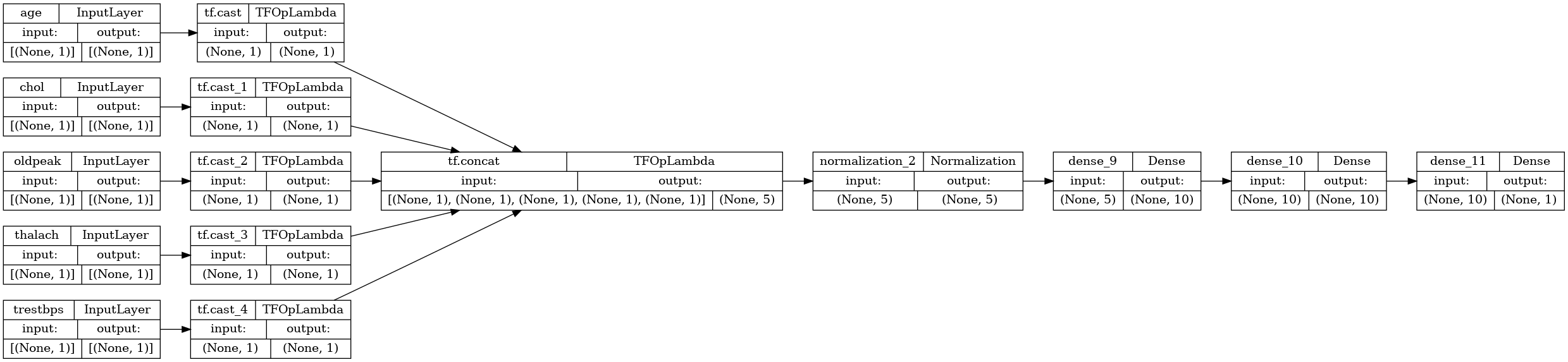
모델 서브 클래스와 동일한 방식으로 기능적 모델을 훈련할 수 있습니다.
model.fit(dict(numeric_features), target, epochs=5, batch_size=BATCH_SIZE)
Epoch 1/5
152/152 [==============================] - 4s 24ms/step - loss: 0.6597 - accuracy: 0.7261
Epoch 2/5
152/152 [==============================] - 4s 23ms/step - loss: 0.5541 - accuracy: 0.7492
Epoch 3/5
152/152 [==============================] - 4s 23ms/step - loss: 0.4860 - accuracy: 0.7558
Epoch 4/5
152/152 [==============================] - 4s 24ms/step - loss: 0.4570 - accuracy: 0.7591
Epoch 5/5
152/152 [==============================] - 4s 24ms/step - loss: 0.4431 - accuracy: 0.7723
<keras.callbacks.History at 0x7f52f5244220>
numeric_dict_batches = numeric_dict_ds.shuffle(SHUFFLE_BUFFER).batch(BATCH_SIZE)
model.fit(numeric_dict_batches, epochs=5)
Epoch 1/5
152/152 [==============================] - 4s 24ms/step - loss: 0.4361 - accuracy: 0.7723
Epoch 2/5
152/152 [==============================] - 4s 25ms/step - loss: 0.4314 - accuracy: 0.7756
Epoch 3/5
152/152 [==============================] - 4s 25ms/step - loss: 0.4298 - accuracy: 0.7822
Epoch 4/5
152/152 [==============================] - 4s 24ms/step - loss: 0.4268 - accuracy: 0.7855
Epoch 5/5
152/152 [==============================] - 4s 24ms/step - loss: 0.4252 - accuracy: 0.7822
<keras.callbacks.History at 0x7f514c58e940>
전체 예제
Keras에 이기종 DataFrame을 전달하는 경우 각 열에 고유한 사전 처리가 필요할 수 있습니다. DataFrame에서 직접 이 전처리를 수행할 수 있지만 모델이 올바르게 작동하려면 입력이 항상 동일한 방식으로 전처리되어야 합니다. 따라서 가장 좋은 방법은 전처리를 모델에 구축하는 것입니다. Keras 전처리 레이어로 많은 일반적인 작업이 처리됩니다.
전처리 헤드 빌드하기
이 데이터세트에서 원시 데이터의 일부 "정수" 특성은 실제로 범주형 인덱스입니다. 이러한 인덱스는 실제로 순서가 지정된 숫자 값이 아닙니다(자세한 내용은 데이터세트 설명 참조). 이것들은 순서가 없기 때문에 모델에 직접 입력하는 것은 부적절합니다. 모델은 이를 순서가 지정된 것으로 해석하기 때문입니다. 이러한 입력을 사용하려면 원-핫 벡터 또는 임베딩 벡터로 인코딩이 필요합니다. 문자열 범주형 특성의 경우도 마찬가지입니다.
참고: 동일한 전처리가 필요한 특성이 많은 경우 전처리를 적용하기 전에 이들을 함께 연결하는 것이 더 효율적입니다.
반면에 이진 특성은 일반적으로 인코딩하거나 정규화할 필요가 없습니다.
먼저 각 그룹에 속하는 특성 목록을 작성합니다.
binary_feature_names = ['sex', 'fbs', 'exang']
categorical_feature_names = ['cp', 'restecg', 'slope', 'thal', 'ca']
다음으로, 각 입력에 적절한 전처리를 적용하고 결과를 연결하는 전처리 모델을 구축합니다.
이 섹션에서는 Keras Functional API를 사용하여 전처리를 구현합니다. 데이터 프레임의 각 열에 대해 하나의 tf.keras.Input을 생성하는 것으로 시작합니다.
inputs = {}
for name, column in df.items():
  if type(column[0]) == str:
    dtype = tf.string
  elif (name in categorical_feature_names or
        name in binary_feature_names):
    dtype = tf.int64
  else:
    dtype = tf.float32

  inputs[name] = tf.keras.Input(shape=(), name=name, dtype=dtype)
inputs
{'age': <KerasTensor: shape=(None,) dtype=float32 (created by layer 'age')>,
 'sex': <KerasTensor: shape=(None,) dtype=int64 (created by layer 'sex')>,
 'cp': <KerasTensor: shape=(None,) dtype=int64 (created by layer 'cp')>,
 'trestbps': <KerasTensor: shape=(None,) dtype=float32 (created by layer 'trestbps')>,
 'chol': <KerasTensor: shape=(None,) dtype=float32 (created by layer 'chol')>,
 'fbs': <KerasTensor: shape=(None,) dtype=int64 (created by layer 'fbs')>,
 'restecg': <KerasTensor: shape=(None,) dtype=int64 (created by layer 'restecg')>,
 'thalach': <KerasTensor: shape=(None,) dtype=float32 (created by layer 'thalach')>,
 'exang': <KerasTensor: shape=(None,) dtype=int64 (created by layer 'exang')>,
 'oldpeak': <KerasTensor: shape=(None,) dtype=float32 (created by layer 'oldpeak')>,
 'slope': <KerasTensor: shape=(None,) dtype=int64 (created by layer 'slope')>,
 'ca': <KerasTensor: shape=(None,) dtype=int64 (created by layer 'ca')>,
 'thal': <KerasTensor: shape=(None,) dtype=string (created by layer 'thal')>}
각 입력에 대해 Keras 레이어와 TensorFlow ops를 사용하여 일부 변환을 적용합니다. 각 특성은 스칼라 배치로 시작합니다(shape=(batch,)). 각각의 출력은 tf.float32 벡터의 배치여야 합니다(shape=(batch, n)). 마지막 단계로 모든 벡터를 함께 연결합니다.
이진 입력
이진 입력은 전처리가 필요하지 않으므로 벡터 축을 추가하고 이를 float32로 캐스팅한 다음 전처리된 입력 목록에 추가하기만 하면 됩니다.
preprocessed = []

for name in binary_feature_names:
  inp = inputs[name]
  inp = inp[:, tf.newaxis]
  float_value = tf.cast(inp, tf.float32)
  preprocessed.append(float_value)

preprocessed
[<KerasTensor: shape=(None, 1) dtype=float32 (created by layer 'tf.cast_5')>,
 <KerasTensor: shape=(None, 1) dtype=float32 (created by layer 'tf.cast_6')>,
 <KerasTensor: shape=(None, 1) dtype=float32 (created by layer 'tf.cast_7')>]
숫자 입력
이전 섹션에서와 같이 이러한 숫자 입력도 사용 전에 tf.keras.layers.Normalization 레이어를 통해 실행해야 할 것입니다. 다만 이번에는 dict로 입력된다는 차이가 있습니다. 아래 코드는 DataFrame에서 숫자 특성을 수집하고 적층한 다음 Normalization.adapt 메서드에 전달합니다.
normalizer = tf.keras.layers.Normalization(axis=-1)
normalizer.adapt(stack_dict(dict(numeric_features)))
아래 코드는 숫자 특성을 적층하고 정규화 계층을 통해 실행합니다.
numeric_inputs = {}
for name in numeric_feature_names:
  numeric_inputs[name]=inputs[name]

numeric_inputs = stack_dict(numeric_inputs)
numeric_normalized = normalizer(numeric_inputs)

preprocessed.append(numeric_normalized)

preprocessed
[<KerasTensor: shape=(None, 1) dtype=float32 (created by layer 'tf.cast_5')>,
 <KerasTensor: shape=(None, 1) dtype=float32 (created by layer 'tf.cast_6')>,
 <KerasTensor: shape=(None, 1) dtype=float32 (created by layer 'tf.cast_7')>,
 <KerasTensor: shape=(None, 5) dtype=float32 (created by layer 'normalization_3')>]
범주형 특성
범주형 특성을 사용하려면 먼저 이를 이진 벡터 또는 임베딩으로 인코딩해야 합니다. 이러한 특성에는 소수의 범주만 포함되어 있으므로 tf.keras.layers.StringLookup 및 tf.keras.layers.IntegerLookup 레이어 모두에서 지원하는 output_mode='one_hot' 옵션을 사용하여 입력을 원-핫 벡터로 직접 변환합니다.
다음은 이러한 레이어가 작동하는 방식의 예입니다.
vocab = ['a','b','c']
lookup = tf.keras.layers.StringLookup(vocabulary=vocab, output_mode='one_hot')
lookup(['c','a','a','b','zzz'])
<tf.Tensor: shape=(5, 4), dtype=float32, numpy=
array([[0., 0., 0., 1.],
       [0., 1., 0., 0.],
       [0., 1., 0., 0.],
       [0., 0., 1., 0.],
       [1., 0., 0., 0.]], dtype=float32)>
vocab = [1,4,7,99]
lookup = tf.keras.layers.IntegerLookup(vocabulary=vocab, output_mode='one_hot')

lookup([-1,4,1])
<tf.Tensor: shape=(3, 5), dtype=float32, numpy=
array([[1., 0., 0., 0., 0.],
       [0., 0., 1., 0., 0.],
       [0., 1., 0., 0., 0.]], dtype=float32)>
각 입력에 대한 어휘를 결정하려면 해당 어휘를 원-핫 벡터로 변환하는 레이어를 만듭니다.
for name in categorical_feature_names:
  vocab = sorted(set(df[name]))
  print(f'name: {name}')
  print(f'vocab: {vocab}\n')

  if type(vocab[0]) is str:
    lookup = tf.keras.layers.StringLookup(vocabulary=vocab, output_mode='one_hot')
  else:
    lookup = tf.keras.layers.IntegerLookup(vocabulary=vocab, output_mode='one_hot')

  x = inputs[name][:, tf.newaxis]
  x = lookup(x)
  preprocessed.append(x)
name: cp
vocab: [0, 1, 2, 3, 4]

name: restecg
vocab: [0, 1, 2]

name: slope
vocab: [1, 2, 3]

name: thal
vocab: ['1', '2', 'fixed', 'normal', 'reversible']

name: ca
vocab: [0, 1, 2, 3]
전처리 헤드 조립하기
이 시점에서 preprocessed는 모든 전처리 결과의 Python 목록일 뿐이며 각 결과의 형상은 (batch_size, depth)입니다.
preprocessed
[<KerasTensor: shape=(None, 1) dtype=float32 (created by layer 'tf.cast_5')>,
 <KerasTensor: shape=(None, 1) dtype=float32 (created by layer 'tf.cast_6')>,
 <KerasTensor: shape=(None, 1) dtype=float32 (created by layer 'tf.cast_7')>,
 <KerasTensor: shape=(None, 5) dtype=float32 (created by layer 'normalization_3')>,
 <KerasTensor: shape=(None, 6) dtype=float32 (created by layer 'integer_lookup_1')>,
 <KerasTensor: shape=(None, 4) dtype=float32 (created by layer 'integer_lookup_2')>,
 <KerasTensor: shape=(None, 4) dtype=float32 (created by layer 'integer_lookup_3')>,
 <KerasTensor: shape=(None, 6) dtype=float32 (created by layer 'string_lookup_1')>,
 <KerasTensor: shape=(None, 5) dtype=float32 (created by layer 'integer_lookup_4')>]
depth 축을 따라 전처리된 모든 특성을 연결하여 각 사전-예제가 단일 벡터로 변환되도록 합니다. 벡터에는 범주형 특성, 숫자 특성 및 범주형 원-핫 특성이 포함됩니다.
preprocesssed_result = tf.concat(preprocessed, axis=-1)
preprocesssed_result
<KerasTensor: shape=(None, 33) dtype=float32 (created by layer 'tf.concat_1')>
이제 해당 계산에서 모델을 생성하여 재사용할 수 있도록 합니다.
preprocessor = tf.keras.Model(inputs, preprocesssed_result)
tf.keras.utils.plot_model(preprocessor, rankdir="LR", show_shapes=True)
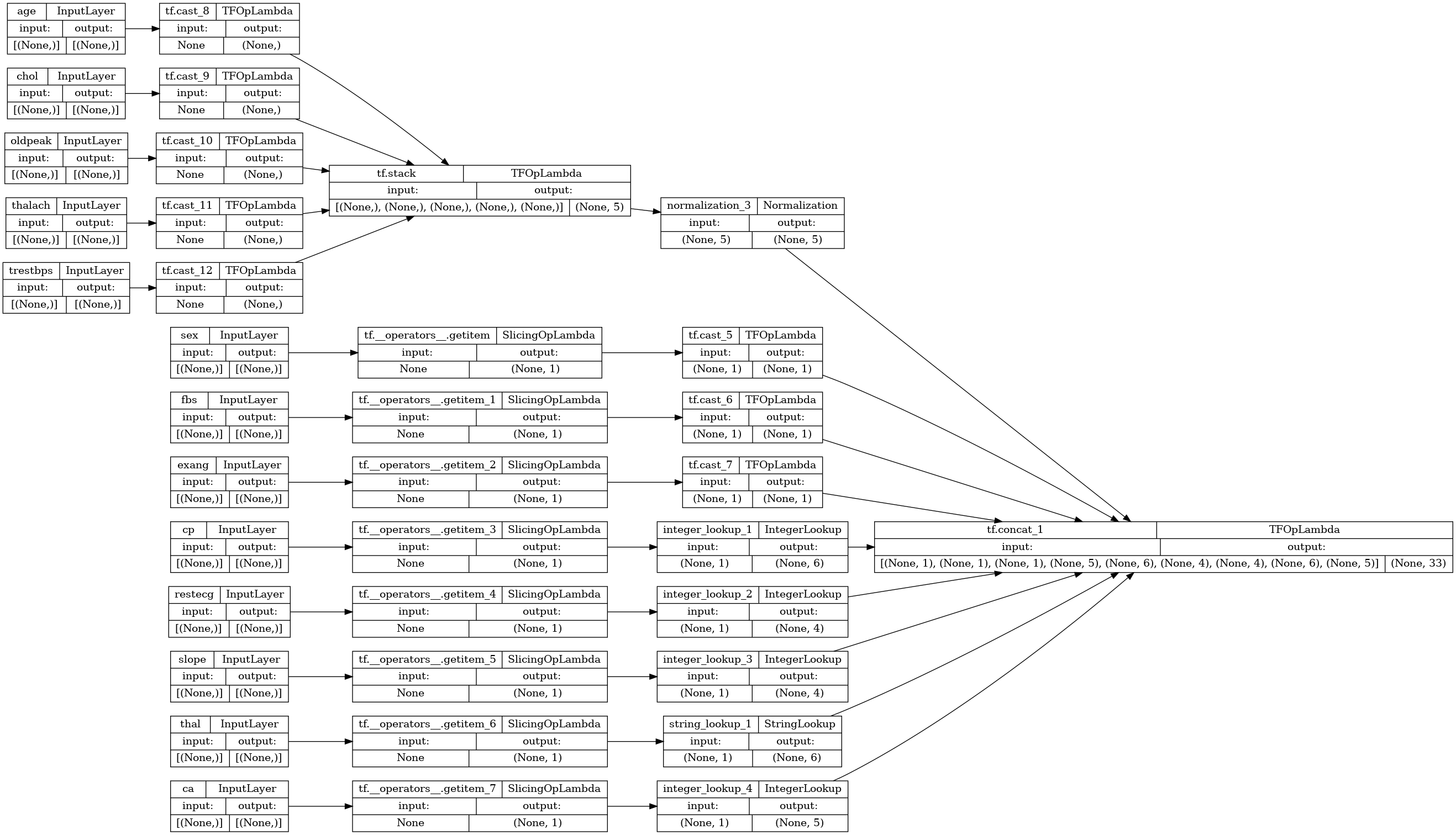
전처리기를 테스트하려면 DataFrame.iloc 접근자를 사용하여 DataFrame에서 첫 번째 예제를 조각화합니다. 그런 다음 이를 사전으로 변환하고 사전을 전처리기에 전달합니다. 결과적으로 얻어지는 것은 이진 특성, 정규화된 숫자 특성 및 원-핫 범주 특성을 순서대로 포함하는 단일 벡터입니다.
preprocessor(dict(df.iloc[:1]))
<tf.Tensor: shape=(1, 33), dtype=float32, numpy=
array([[ 1.        ,  1.        ,  0.        ,  0.93383914, -0.26008663,
         1.0680453 ,  0.03480718,  0.74578077,  0.        ,  0.        ,

         1.        ,  0.        ,  0.        ,  0.        ,  0.        ,
         0.        ,  0.        ,  1.        ,  0.        ,  0.        ,
         0.        ,  1.        ,  0.        ,  0.        ,  0.        ,
         1.        ,  0.        ,  0.        ,  0.        ,  1.        ,
         0.        ,  0.        ,  0.        ]], dtype=float32)>
모델 생성 및 훈련
이제 모델의 본문을 만듭니다. 이전 예와 동일한 구성을 사용합니다. 바로, 몇 개의 Dense rectified-linear 레이어와 분류를 위한 Dense(1) 출력 레이어입니다.
body = tf.keras.Sequential([
  tf.keras.layers.Dense(10, activation='relu'),
  tf.keras.layers.Dense(10, activation='relu'),
  tf.keras.layers.Dense(1)
])
이제 Keras functional API를 사용하여 두 조각을 함께 연결합니다.
inputs
{'age': <KerasTensor: shape=(None,) dtype=float32 (created by layer 'age')>,
 'sex': <KerasTensor: shape=(None,) dtype=int64 (created by layer 'sex')>,
 'cp': <KerasTensor: shape=(None,) dtype=int64 (created by layer 'cp')>,
 'trestbps': <KerasTensor: shape=(None,) dtype=float32 (created by layer 'trestbps')>,
 'chol': <KerasTensor: shape=(None,) dtype=float32 (created by layer 'chol')>,
 'fbs': <KerasTensor: shape=(None,) dtype=int64 (created by layer 'fbs')>,
 'restecg': <KerasTensor: shape=(None,) dtype=int64 (created by layer 'restecg')>,
 'thalach': <KerasTensor: shape=(None,) dtype=float32 (created by layer 'thalach')>,
 'exang': <KerasTensor: shape=(None,) dtype=int64 (created by layer 'exang')>,
 'oldpeak': <KerasTensor: shape=(None,) dtype=float32 (created by layer 'oldpeak')>,
 'slope': <KerasTensor: shape=(None,) dtype=int64 (created by layer 'slope')>,
 'ca': <KerasTensor: shape=(None,) dtype=int64 (created by layer 'ca')>,
 'thal': <KerasTensor: shape=(None,) dtype=string (created by layer 'thal')>}
x = preprocessor(inputs)
x
<KerasTensor: shape=(None, 33) dtype=float32 (created by layer 'model_1')>
result = body(x)
result
<KerasTensor: shape=(None, 1) dtype=float32 (created by layer 'sequential_3')>
model = tf.keras.Model(inputs, result)

model.compile(optimizer='adam',
                loss=tf.keras.losses.BinaryCrossentropy(from_logits=True),
                metrics=['accuracy'])
이 모델은 입력 사전을 예상합니다. 데이터를 전달하는 가장 간단한 방법은 DataFrame을 dict로 변환하고 해당 dict를 Model.fit에 x 인수로 전달하는 것입니다.
history = model.fit(dict(df), target, epochs=5, batch_size=BATCH_SIZE)
Epoch 1/5
152/152 [==============================] - 2s 5ms/step - loss: 0.5852 - accuracy: 0.7261
Epoch 2/5
152/152 [==============================] - 1s 4ms/step - loss: 0.4585 - accuracy: 0.7657
Epoch 3/5
152/152 [==============================] - 1s 5ms/step - loss: 0.3868 - accuracy: 0.7756
Epoch 4/5
152/152 [==============================] - 1s 5ms/step - loss: 0.3471 - accuracy: 0.8119
Epoch 5/5
152/152 [==============================] - 1s 5ms/step - loss: 0.3270 - accuracy: 0.8185
tf.data를 사용해도 됩니다.
ds = tf.data.Dataset.from_tensor_slices((
    dict(df),
    target
))

ds = ds.batch(BATCH_SIZE)
import pprint

for x, y in ds.take(1):
  pprint.pprint(x)
  print()
  print(y)
{'age': <tf.Tensor: shape=(2,), dtype=int64, numpy=array([63, 67])>,
 'ca': <tf.Tensor: shape=(2,), dtype=int64, numpy=array([0, 3])>,
 'chol': <tf.Tensor: shape=(2,), dtype=int64, numpy=array([233, 286])>,
 'cp': <tf.Tensor: shape=(2,), dtype=int64, numpy=array([1, 4])>,
 'exang': <tf.Tensor: shape=(2,), dtype=int64, numpy=array([0, 1])>,
 'fbs': <tf.Tensor: shape=(2,), dtype=int64, numpy=array([1, 0])>,
 'oldpeak': <tf.Tensor: shape=(2,), dtype=float64, numpy=array([2.3, 1.5])>,
 'restecg': <tf.Tensor: shape=(2,), dtype=int64, numpy=array([2, 2])>,
 'sex': <tf.Tensor: shape=(2,), dtype=int64, numpy=array([1, 1])>,
 'slope': <tf.Tensor: shape=(2,), dtype=int64, numpy=array([3, 2])>,
 'thal': <tf.Tensor: shape=(2,), dtype=string, numpy=array([b'fixed', b'normal'], dtype=object)>,
 'thalach': <tf.Tensor: shape=(2,), dtype=int64, numpy=array([150, 108])>,
 'trestbps': <tf.Tensor: shape=(2,), dtype=int64, numpy=array([145, 160])>}

tf.Tensor([0 1], shape=(2,), dtype=int64)
history = model.fit(ds, epochs=5)
Epoch 1/5
152/152 [==============================] - 1s 4ms/step - loss: 0.3107 - accuracy: 0.8548
Epoch 2/5
152/152 [==============================] - 1s 4ms/step - loss: 0.2972 - accuracy: 0.8548
Epoch 3/5
152/152 [==============================] - 1s 5ms/step - loss: 0.2870 - accuracy: 0.8647
Epoch 4/5
152/152 [==============================] - 1s 5ms/step - loss: 0.2784 - accuracy: 0.8614
Epoch 5/5
152/152 [==============================] - 1s 4ms/step - loss: 0.2704 - accuracy: 0.8581