
|
|
|
 在 GitHub 上查看源代码
|
|
此笔记本训练一个将西班牙语翻译为英语的序列到序列(sequence to sequence,简写为 seq2seq)模型。此例子难度较高,需要对序列到序列模型的知识有一定了解。
训练完此笔记本中的模型后,你将能够输入一个西班牙语句子,例如 "¿todavia estan en casa?",并返回其英语翻译 "are you still at home?"
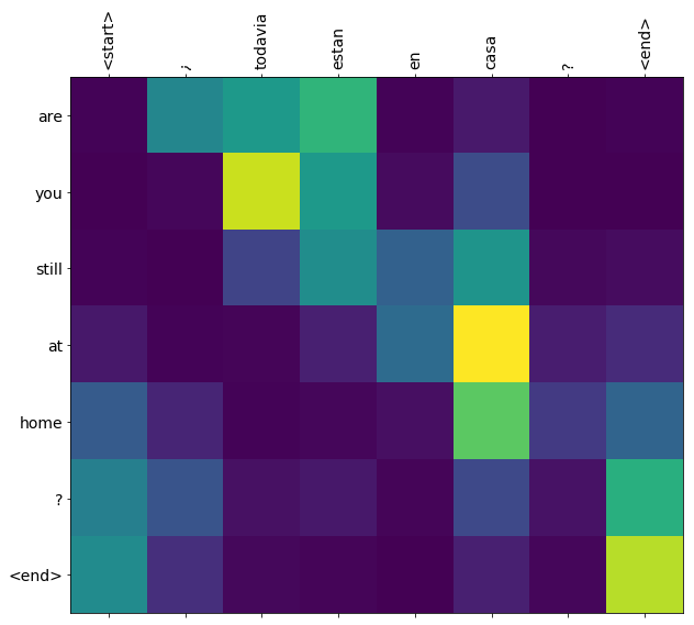
对于一个简单的例子来说,翻译质量令人满意。但是更有趣的可能是生成的注意力图:它显示在翻译过程中,输入句子的哪些部分受到了模型的注意。
请注意:运行这个例子用一个 P100 GPU 需要花大约 10 分钟。
import tensorflow as tf

import matplotlib.pyplot as plt
import matplotlib.ticker as ticker
from sklearn.model_selection import train_test_split

import unicodedata
import re
import numpy as np
import os
import io
import time
下载和准备数据集
我们将使用 http://www.manythings.org/anki/ 提供的一个语言数据集。这个数据集包含如下格式的语言翻译对:
May I borrow this book? ¿Puedo tomar prestado este libro?
这个数据集中有很多种语言可供选择。我们将使用英语 - 西班牙语数据集。为方便使用,我们在谷歌云上提供了此数据集的一份副本。但是你也可以自己下载副本。下载完数据集后,我们将采取下列步骤准备数据:
- 给每个句子添加一个 开始 和一个 结束 标记(token)。
- 删除特殊字符以清理句子。
- 创建一个单词索引和一个反向单词索引(即一个从单词映射至 id 的词典和一个从 id 映射至单词的词典)。
- 将每个句子填充(pad)到最大长度。
# 下载文件
path_to_zip = tf.keras.utils.get_file(
    'spa-eng.zip', origin='http://storage.googleapis.com/download.tensorflow.org/data/spa-eng.zip',
    extract=True)

path_to_file = os.path.dirname(path_to_zip)+"/spa-eng/spa.txt"
# 将 unicode 文件转换为 ascii
def unicode_to_ascii(s):
    return ''.join(c for c in unicodedata.normalize('NFD', s)
        if unicodedata.category(c) != 'Mn')


def preprocess_sentence(w):
    w = unicode_to_ascii(w.lower().strip())

    # 在单词与跟在其后的标点符号之间插入一个空格
    # 例如: "he is a boy." => "he is a boy ."
    # 参考:https://stackoverflow.com/questions/3645931/python-padding-punctuation-with-white-spaces-keeping-punctuation
    w = re.sub(r"([?.!,¿])", r" \1 ", w)
    w = re.sub(r'[" "]+', " ", w)

    # 除了 (a-z, A-Z, ".", "?", "!", ","),将所有字符替换为空格
    w = re.sub(r"[^a-zA-Z?.!,¿]+", " ", w)

    w = w.rstrip().strip()

    # 给句子加上开始和结束标记
    # 以便模型知道何时开始和结束预测
    w = '<start> ' + w + ' <end>'
    return w
en_sentence = u"May I borrow this book?"
sp_sentence = u"¿Puedo tomar prestado este libro?"
print(preprocess_sentence(en_sentence))
print(preprocess_sentence(sp_sentence).encode('utf-8'))
# 1. 去除重音符号
# 2. 清理句子
# 3. 返回这样格式的单词对:[ENGLISH, SPANISH]
def create_dataset(path, num_examples):
    lines = io.open(path, encoding='UTF-8').read().strip().split('\n')

    word_pairs = [[preprocess_sentence(w) for w in l.split('\t')]  for l in lines[:num_examples]]

    return zip(*word_pairs)
en, sp = create_dataset(path_to_file, None)
print(en[-1])
print(sp[-1])
def max_length(tensor):
    return max(len(t) for t in tensor)
def tokenize(lang):
  lang_tokenizer = tf.keras.preprocessing.text.Tokenizer(
      filters='')
  lang_tokenizer.fit_on_texts(lang)

  tensor = lang_tokenizer.texts_to_sequences(lang)

  tensor = tf.keras.preprocessing.sequence.pad_sequences(tensor,
                                                         padding='post')

  return tensor, lang_tokenizer
def load_dataset(path, num_examples=None):
    # 创建清理过的输入输出对
    targ_lang, inp_lang = create_dataset(path, num_examples)

    input_tensor, inp_lang_tokenizer = tokenize(inp_lang)
    target_tensor, targ_lang_tokenizer = tokenize(targ_lang)

    return input_tensor, target_tensor, inp_lang_tokenizer, targ_lang_tokenizer
限制数据集的大小以加快实验速度(可选)
在超过 10 万个句子的完整数据集上训练需要很长时间。为了更快地训练,我们可以将数据集的大小限制为 3 万个句子(当然,翻译质量也会随着数据的减少而降低):
# 尝试实验不同大小的数据集
num_examples = 30000
input_tensor, target_tensor, inp_lang, targ_lang = load_dataset(path_to_file, num_examples)

# 计算目标张量的最大长度 (max_length)
max_length_targ, max_length_inp = max_length(target_tensor), max_length(input_tensor)
# 采用 80 - 20 的比例切分训练集和验证集
input_tensor_train, input_tensor_val, target_tensor_train, target_tensor_val = train_test_split(input_tensor, target_tensor, test_size=0.2)

# 显示长度
print(len(input_tensor_train), len(target_tensor_train), len(input_tensor_val), len(target_tensor_val))
def convert(lang, tensor):
  for t in tensor:
    if t!=0:
      print ("%d ----> %s" % (t, lang.index_word[t]))
print ("Input Language; index to word mapping")
convert(inp_lang, input_tensor_train[0])
print ()
print ("Target Language; index to word mapping")
convert(targ_lang, target_tensor_train[0])
创建一个 tf.data 数据集
BUFFER_SIZE = len(input_tensor_train)
BATCH_SIZE = 64
steps_per_epoch = len(input_tensor_train)//BATCH_SIZE
embedding_dim = 256
units = 1024
vocab_inp_size = len(inp_lang.word_index)+1
vocab_tar_size = len(targ_lang.word_index)+1

dataset = tf.data.Dataset.from_tensor_slices((input_tensor_train, target_tensor_train)).shuffle(BUFFER_SIZE)
dataset = dataset.batch(BATCH_SIZE, drop_remainder=True)
example_input_batch, example_target_batch = next(iter(dataset))
example_input_batch.shape, example_target_batch.shape
编写编码器 (encoder) 和解码器 (decoder) 模型
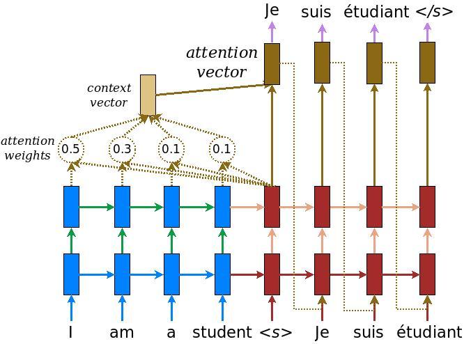
实现一个基于注意力的编码器 - 解码器模型。关于这种模型,你可以阅读 TensorFlow 的 神经机器翻译 (序列到序列) 教程。本示例采用一组更新的 API。此笔记本实现了上述序列到序列教程中的 注意力方程式。下图显示了注意力机制为每个输入单词分配一个权重,然后解码器将这个权重用于预测句子中的下一个单词。下图和公式是 Luong 的论文中注意力机制的一个例子。
输入经过编码器模型,编码器模型为我们提供形状为 (批大小,最大长度,隐藏层大小) 的编码器输出和形状为 (批大小,隐藏层大小) 的编码器隐藏层状态。
下面是所实现的方程式:
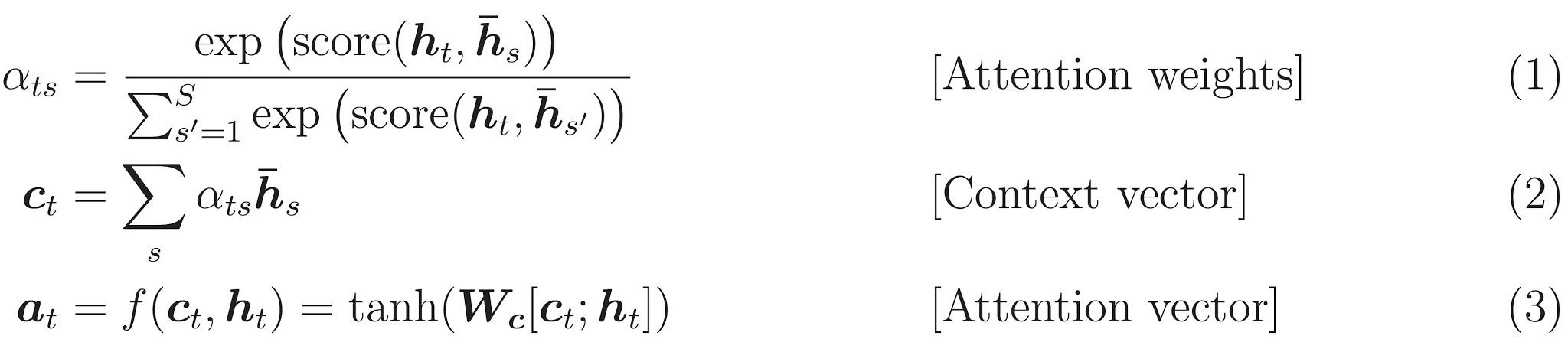
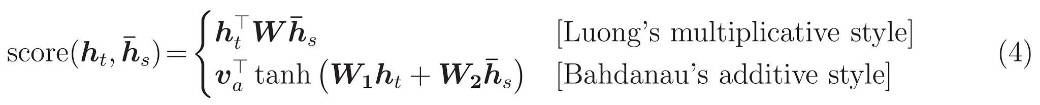
本教程的编码器采用 Bahdanau 注意力。在用简化形式编写之前,让我们先决定符号:
- FC = 完全连接(密集)层
- EO = 编码器输出
- H = 隐藏层状态
- X = 解码器输入
以及伪代码:
score = FC(tanh(FC(EO) + FC(H)))attention weights = softmax(score, axis = 1)。 Softmax 默认被应用于最后一个轴,但是这里我们想将它应用于 第一个轴, 因为分数 (score) 的形状是 (批大小,最大长度,隐藏层大小)。最大长度 (max_length) 是我们的输入的长度。因为我们想为每个输入分配一个权重,所以 softmax 应该用在这个轴上。context vector = sum(attention weights * EO, axis = 1)。选择第一个轴的原因同上。embedding output= 解码器输入 X 通过一个嵌入层。merged vector = concat(embedding output, context vector)- 此合并后的向量随后被传送到 GRU
每个步骤中所有向量的形状已在代码的注释中阐明:
class Encoder(tf.keras.Model):
  def __init__(self, vocab_size, embedding_dim, enc_units, batch_sz):
    super(Encoder, self).__init__()
    self.batch_sz = batch_sz
    self.enc_units = enc_units
    self.embedding = tf.keras.layers.Embedding(vocab_size, embedding_dim)
    self.gru = tf.keras.layers.GRU(self.enc_units,
                                   return_sequences=True,
                                   return_state=True,
                                   recurrent_initializer='glorot_uniform')

  def call(self, x, hidden):
    x = self.embedding(x)
    output, state = self.gru(x, initial_state = hidden)
    return output, state

  def initialize_hidden_state(self):
    return tf.zeros((self.batch_sz, self.enc_units))
encoder = Encoder(vocab_inp_size, embedding_dim, units, BATCH_SIZE)

# 样本输入
sample_hidden = encoder.initialize_hidden_state()
sample_output, sample_hidden = encoder(example_input_batch, sample_hidden)
print ('Encoder output shape: (batch size, sequence length, units) {}'.format(sample_output.shape))
print ('Encoder Hidden state shape: (batch size, units) {}'.format(sample_hidden.shape))
class BahdanauAttention(tf.keras.layers.Layer):
  def __init__(self, units):
    super(BahdanauAttention, self).__init__()
    self.W1 = tf.keras.layers.Dense(units)
    self.W2 = tf.keras.layers.Dense(units)
    self.V = tf.keras.layers.Dense(1)

  def call(self, query, values):
    # 隐藏层的形状 == (批大小,隐藏层大小)
    # hidden_with_time_axis 的形状 == (批大小,1,隐藏层大小)
    # 这样做是为了执行加法以计算分数
    hidden_with_time_axis = tf.expand_dims(query, 1)

    # 分数的形状 == (批大小,最大长度,1)
    # 我们在最后一个轴上得到 1, 因为我们把分数应用于 self.V
    # 在应用 self.V 之前,张量的形状是(批大小,最大长度,单位)
    score = self.V(tf.nn.tanh(
        self.W1(values) + self.W2(hidden_with_time_axis)))

    # 注意力权重 (attention_weights) 的形状 == (批大小,最大长度,1)
    attention_weights = tf.nn.softmax(score, axis=1)

    # 上下文向量 (context_vector) 求和之后的形状 == (批大小,隐藏层大小)
    context_vector = attention_weights * values
    context_vector = tf.reduce_sum(context_vector, axis=1)

    return context_vector, attention_weights
attention_layer = BahdanauAttention(10)
attention_result, attention_weights = attention_layer(sample_hidden, sample_output)

print("Attention result shape: (batch size, units) {}".format(attention_result.shape))
print("Attention weights shape: (batch_size, sequence_length, 1) {}".format(attention_weights.shape))
class Decoder(tf.keras.Model):
  def __init__(self, vocab_size, embedding_dim, dec_units, batch_sz):
    super(Decoder, self).__init__()
    self.batch_sz = batch_sz
    self.dec_units = dec_units
    self.embedding = tf.keras.layers.Embedding(vocab_size, embedding_dim)
    self.gru = tf.keras.layers.GRU(self.dec_units,
                                   return_sequences=True,
                                   return_state=True,
                                   recurrent_initializer='glorot_uniform')
    self.fc = tf.keras.layers.Dense(vocab_size)

    # 用于注意力
    self.attention = BahdanauAttention(self.dec_units)

  def call(self, x, hidden, enc_output):
    # 编码器输出 (enc_output) 的形状 == (批大小,最大长度,隐藏层大小)
    context_vector, attention_weights = self.attention(hidden, enc_output)

    # x 在通过嵌入层后的形状 == (批大小,1,嵌入维度)
    x = self.embedding(x)

    # x 在拼接 (concatenation) 后的形状 == (批大小,1,嵌入维度 + 隐藏层大小)
    x = tf.concat([tf.expand_dims(context_vector, 1), x], axis=-1)

    # 将合并后的向量传送到 GRU
    output, state = self.gru(x)

    # 输出的形状 == (批大小 * 1,隐藏层大小)
    output = tf.reshape(output, (-1, output.shape[2]))

    # 输出的形状 == (批大小,vocab)
    x = self.fc(output)

    return x, state, attention_weights
decoder = Decoder(vocab_tar_size, embedding_dim, units, BATCH_SIZE)

sample_decoder_output, _, _ = decoder(tf.random.uniform((64, 1)),
                                      sample_hidden, sample_output)

print ('Decoder output shape: (batch_size, vocab size) {}'.format(sample_decoder_output.shape))
定义优化器和损失函数
optimizer = tf.keras.optimizers.Adam()
loss_object = tf.keras.losses.SparseCategoricalCrossentropy(
    from_logits=True, reduction='none')

def loss_function(real, pred):
  mask = tf.math.logical_not(tf.math.equal(real, 0))
  loss_ = loss_object(real, pred)

  mask = tf.cast(mask, dtype=loss_.dtype)
  loss_ *= mask

  return tf.reduce_mean(loss_)
检查点(基于对象保存)
checkpoint_dir = './training_checkpoints'
checkpoint_prefix = os.path.join(checkpoint_dir, "ckpt")
checkpoint = tf.train.Checkpoint(optimizer=optimizer,
                                 encoder=encoder,
                                 decoder=decoder)
训练
- 将 输入 传送至 编码器,编码器返回 编码器输出 和 编码器隐藏层状态。
- 将编码器输出、编码器隐藏层状态和解码器输入(即 开始标记)传送至解码器。
- 解码器返回 预测 和 解码器隐藏层状态。
- 解码器隐藏层状态被传送回模型,预测被用于计算损失。
- 使用 教师强制 (teacher forcing) 决定解码器的下一个输入。
- 教师强制 是将 目标词 作为 下一个输入 传送至解码器的技术。
- 最后一步是计算梯度,并将其应用于优化器和反向传播。
@tf.function
def train_step(inp, targ, enc_hidden):
  loss = 0

  with tf.GradientTape() as tape:
    enc_output, enc_hidden = encoder(inp, enc_hidden)

    dec_hidden = enc_hidden

    dec_input = tf.expand_dims([targ_lang.word_index['<start>']] * BATCH_SIZE, 1)

    # 教师强制 - 将目标词作为下一个输入
    for t in range(1, targ.shape[1]):
      # 将编码器输出 (enc_output) 传送至解码器
      predictions, dec_hidden, _ = decoder(dec_input, dec_hidden, enc_output)

      loss += loss_function(targ[:, t], predictions)

      # 使用教师强制
      dec_input = tf.expand_dims(targ[:, t], 1)

  batch_loss = (loss / int(targ.shape[1]))

  variables = encoder.trainable_variables + decoder.trainable_variables

  gradients = tape.gradient(loss, variables)

  optimizer.apply_gradients(zip(gradients, variables))

  return batch_loss
EPOCHS = 10

for epoch in range(EPOCHS):
  start = time.time()

  enc_hidden = encoder.initialize_hidden_state()
  total_loss = 0

  for (batch, (inp, targ)) in enumerate(dataset.take(steps_per_epoch)):
    batch_loss = train_step(inp, targ, enc_hidden)
    total_loss += batch_loss

    if batch % 100 == 0:
        print('Epoch {} Batch {} Loss {:.4f}'.format(epoch + 1,
                                                     batch,
                                                     batch_loss.numpy()))
  # 每 2 个周期(epoch),保存(检查点)一次模型
  if (epoch + 1) % 2 == 0:
    checkpoint.save(file_prefix = checkpoint_prefix)

  print('Epoch {} Loss {:.4f}'.format(epoch + 1,
                                      total_loss / steps_per_epoch))
  print('Time taken for 1 epoch {} sec\n'.format(time.time() - start))
翻译
- 评估函数类似于训练循环,不同之处在于在这里我们不使用 教师强制。每个时间步的解码器输入是其先前的预测、隐藏层状态和编码器输出。
- 当模型预测 结束标记 时停止预测。
- 存储 每个时间步的注意力权重。
请注意:对于一个输入,编码器输出仅计算一次。
def evaluate(sentence):
    attention_plot = np.zeros((max_length_targ, max_length_inp))

    sentence = preprocess_sentence(sentence)

    inputs = [inp_lang.word_index[i] for i in sentence.split(' ')]
    inputs = tf.keras.preprocessing.sequence.pad_sequences([inputs],
                                                           maxlen=max_length_inp,
                                                           padding='post')
    inputs = tf.convert_to_tensor(inputs)

    result = ''

    hidden = [tf.zeros((1, units))]
    enc_out, enc_hidden = encoder(inputs, hidden)

    dec_hidden = enc_hidden
    dec_input = tf.expand_dims([targ_lang.word_index['<start>']], 0)

    for t in range(max_length_targ):
        predictions, dec_hidden, attention_weights = decoder(dec_input,
                                                             dec_hidden,
                                                             enc_out)

        # 存储注意力权重以便后面制图
        attention_weights = tf.reshape(attention_weights, (-1, ))
        attention_plot[t] = attention_weights.numpy()

        predicted_id = tf.argmax(predictions[0]).numpy()

        result += targ_lang.index_word[predicted_id] + ' '

        if targ_lang.index_word[predicted_id] == '<end>':
            return result, sentence, attention_plot

        # 预测的 ID 被输送回模型
        dec_input = tf.expand_dims([predicted_id], 0)

    return result, sentence, attention_plot
# 注意力权重制图函数
def plot_attention(attention, sentence, predicted_sentence):
    fig = plt.figure(figsize=(10,10))
    ax = fig.add_subplot(1, 1, 1)
    ax.matshow(attention, cmap='viridis')

    fontdict = {'fontsize': 14}

    ax.set_xticklabels([''] + sentence, fontdict=fontdict, rotation=90)
    ax.set_yticklabels([''] + predicted_sentence, fontdict=fontdict)

    ax.xaxis.set_major_locator(ticker.MultipleLocator(1))
    ax.yaxis.set_major_locator(ticker.MultipleLocator(1))

    plt.show()
def translate(sentence):
    result, sentence, attention_plot = evaluate(sentence)

    print('Input: %s' % (sentence))
    print('Predicted translation: {}'.format(result))

    attention_plot = attention_plot[:len(result.split(' ')), :len(sentence.split(' '))]
    plot_attention(attention_plot, sentence.split(' '), result.split(' '))
恢复最新的检查点并验证
# 恢复检查点目录 (checkpoint_dir) 中最新的检查点
checkpoint.restore(tf.train.latest_checkpoint(checkpoint_dir))
translate(u'hace mucho frio aqui.')
translate(u'esta es mi vida.')
translate(u'¿todavia estan en casa?')
# 错误的翻译
translate(u'trata de averiguarlo.')
下一步
- 下载一个不同的数据集实验翻译,例如英语到德语或者英语到法语。
- 实验在更大的数据集上训练,或者增加训练周期。