
| | |  Xem trên GitHub Xem trên GitHub | | |
Phân loại máy tính xách tay Bộ phim này đánh giá là tích cực hay tiêu cực bằng cách sử dụng văn bản của tổng quan. Đây là một ví dụ về nhị phân -Hoặc hai đẳng cấp phân loại, một loại quan trọng và được áp dụng rộng rãi của máy có vấn đề học tập.
Chúng tôi sẽ sử dụng các dữ liệu IMDB có chứa nội dung của 50.000 đánh giá phim từ Internet Movie Database . Chúng được chia thành 25.000 đánh giá để đào tạo và 25.000 đánh giá để kiểm tra. Việc đào tạo và thử nghiệm bộ được cân bằng, nghĩa là chúng có chứa một số lượng tương đương đánh giá tích cực và tiêu cực.
Máy tính xách tay này sử dụng tf.keras , một API cấp cao để xây dựng và đào tạo mô hình trong TensorFlow, và TensorFlow Hub , một thư viện và nền tảng cho việc học chuyển tiếp. Đối với một văn bản tiên tiến hơn phân loại hướng dẫn sử dụng tf.keras , xem chữ MLCC Phân Hướng dẫn .
Nhiều mô hình hơn
Ở đây bạn có thể tìm mô hình biểu cảm nhiều hơn hoặc performant mà bạn có thể sử dụng để tạo ra nhúng văn bản.
Thành lập
import numpy as np

import tensorflow as tf
import tensorflow_hub as hub
import tensorflow_datasets as tfds

import matplotlib.pyplot as plt

print("Version: ", tf.__version__)
print("Eager mode: ", tf.executing_eagerly())
print("Hub version: ", hub.__version__)
print("GPU is", "available" if tf.config.list_physical_devices('GPU') else "NOT AVAILABLE")
Version:  2.7.0
Eager mode:  True
Hub version:  0.12.0
GPU is available
Tải xuống tập dữ liệu IMDB
Bộ dữ liệu IMDB có sẵn trên bộ dữ liệu TensorFlow . Đoạn mã sau tải tập dữ liệu IMDB xuống máy của bạn (hoặc thời gian chạy colab):
train_data, test_data = tfds.load(name="imdb_reviews", split=["train", "test"],
                                  batch_size=-1, as_supervised=True)

train_examples, train_labels = tfds.as_numpy(train_data)
test_examples, test_labels = tfds.as_numpy(test_data)
WARNING:tensorflow:From /tmpfs/src/tf_docs_env/lib/python3.7/site-packages/tensorflow_datasets/core/dataset_builder.py:622: get_single_element (from tensorflow.python.data.experimental.ops.get_single_element) is deprecated and will be removed in a future version.
Instructions for updating:
Use `tf.data.Dataset.get_single_element()`.
Khám phá dữ liệu
Hãy dành một chút thời gian để hiểu định dạng của dữ liệu. Mỗi ví dụ là một câu đại diện cho bài đánh giá phim và một nhãn tương ứng. Câu không được xử lý trước theo bất kỳ cách nào. Nhãn là một giá trị nguyên của 0 hoặc 1, trong đó 0 là đánh giá tiêu cực và 1 là đánh giá tích cực.
print("Training entries: {}, test entries: {}".format(len(train_examples), len(test_examples)))
Training entries: 25000, test entries: 25000
Hãy in 10 ví dụ đầu tiên.
train_examples[:10]
array([b"This was an absolutely terrible movie. Don't be lured in by Christopher Walken or Michael Ironside. Both are great actors, but this must simply be their worst role in history. Even their great acting could not redeem this movie's ridiculous storyline. This movie is an early nineties US propaganda piece. The most pathetic scenes were those when the Columbian rebels were making their cases for revolutions. Maria Conchita Alonso appeared phony, and her pseudo-love affair with Walken was nothing but a pathetic emotional plug in a movie that was devoid of any real meaning. I am disappointed that there are movies like this, ruining actor's like Christopher Walken's good name. I could barely sit through it.",
       b'I have been known to fall asleep during films, but this is usually due to a combination of things including, really tired, being warm and comfortable on the sette and having just eaten a lot. However on this occasion I fell asleep because the film was rubbish. The plot development was constant. Constantly slow and boring. Things seemed to happen, but with no explanation of what was causing them or why. I admit, I may have missed part of the film, but i watched the majority of it and everything just seemed to happen of its own accord without any real concern for anything else. I cant recommend this film at all.',
       b'Mann photographs the Alberta Rocky Mountains in a superb fashion, and Jimmy Stewart and Walter Brennan give enjoyable performances as they always seem to do. <br /><br />But come on Hollywood - a Mountie telling the people of Dawson City, Yukon to elect themselves a marshal (yes a marshal!) and to enforce the law themselves, then gunfighters battling it out on the streets for control of the town? <br /><br />Nothing even remotely resembling that happened on the Canadian side of the border during the Klondike gold rush. Mr. Mann and company appear to have mistaken Dawson City for Deadwood, the Canadian North for the American Wild West.<br /><br />Canadian viewers be prepared for a Reefer Madness type of enjoyable howl with this ludicrous plot, or, to shake your head in disgust.',
       b'This is the kind of film for a snowy Sunday afternoon when the rest of the world can go ahead with its own business as you descend into a big arm-chair and mellow for a couple of hours. Wonderful performances from Cher and Nicolas Cage (as always) gently row the plot along. There are no rapids to cross, no dangerous waters, just a warm and witty paddle through New York life at its best. A family film in every sense and one that deserves the praise it received.',
       b'As others have mentioned, all the women that go nude in this film are mostly absolutely gorgeous. The plot very ably shows the hypocrisy of the female libido. When men are around they want to be pursued, but when no "men" are around, they become the pursuers of a 14 year old boy. And the boy becomes a man really fast (we should all be so lucky at this age!). He then gets up the courage to pursue his true love.',
       b"This is a film which should be seen by anybody interested in, effected by, or suffering from an eating disorder. It is an amazingly accurate and sensitive portrayal of bulimia in a teenage girl, its causes and its symptoms. The girl is played by one of the most brilliant young actresses working in cinema today, Alison Lohman, who was later so spectacular in 'Where the Truth Lies'. I would recommend that this film be shown in all schools, as you will never see a better on this subject. Alison Lohman is absolutely outstanding, and one marvels at her ability to convey the anguish of a girl suffering from this compulsive disorder. If barometers tell us the air pressure, Alison Lohman tells us the emotional pressure with the same degree of accuracy. Her emotional range is so precise, each scene could be measured microscopically for its gradations of trauma, on a scale of rising hysteria and desperation which reaches unbearable intensity. Mare Winningham is the perfect choice to play her mother, and does so with immense sympathy and a range of emotions just as finely tuned as Lohman's. Together, they make a pair of sensitive emotional oscillators vibrating in resonance with one another. This film is really an astonishing achievement, and director Katt Shea should be proud of it. The only reason for not seeing it is if you are not interested in people. But even if you like nature films best, this is after all animal behaviour at the sharp edge. Bulimia is an extreme version of how a tormented soul can destroy her own body in a frenzy of despair. And if we don't sympathise with people suffering from the depths of despair, then we are dead inside.",
       b'Okay, you have:<br /><br />Penelope Keith as Miss Herringbone-Tweed, B.B.E. (Backbone of England.) She\'s killed off in the first scene - that\'s right, folks; this show has no backbone!<br /><br />Peter O\'Toole as Ol\' Colonel Cricket from The First War and now the emblazered Lord of the Manor.<br /><br />Joanna Lumley as the ensweatered Lady of the Manor, 20 years younger than the colonel and 20 years past her own prime but still glamourous (Brit spelling, not mine) enough to have a toy-boy on the side. It\'s alright, they have Col. Cricket\'s full knowledge and consent (they guy even comes \'round for Christmas!) Still, she\'s considerate of the colonel enough to have said toy-boy her own age (what a gal!)<br /><br />David McCallum as said toy-boy, equally as pointlessly glamourous as his squeeze. Pilcher couldn\'t come up with any cover for him within the story, so she gave him a hush-hush job at the Circus.<br /><br />and finally:<br /><br />Susan Hampshire as Miss Polonia Teacups, Venerable Headmistress of the Venerable Girls\' Boarding-School, serving tea in her office with a dash of deep, poignant advice for life in the outside world just before graduation. Her best bit of advice: "I\'ve only been to Nancherrow (the local Stately Home of England) once. I thought it was very beautiful but, somehow, not part of the real world." Well, we can\'t say they didn\'t warn us.<br /><br />Ah, Susan - time was, your character would have been running the whole show. They don\'t write \'em like that any more. Our loss, not yours.<br /><br />So - with a cast and setting like this, you have the re-makings of "Brideshead Revisited," right?<br /><br />Wrong! They took these 1-dimensional supporting roles because they paid so well. After all, acting is one of the oldest temp-jobs there is (YOU name another!)<br /><br />First warning sign: lots and lots of backlighting. They get around it by shooting outdoors - "hey, it\'s just the sunlight!"<br /><br />Second warning sign: Leading Lady cries a lot. When not crying, her eyes are moist. That\'s the law of romance novels: Leading Lady is "dewy-eyed."<br /><br />Henceforth, Leading Lady shall be known as L.L.<br /><br />Third warning sign: L.L. actually has stars in her eyes when she\'s in love. Still, I\'ll give Emily Mortimer an award just for having to act with that spotlight in her eyes (I wonder . did they use contacts?)<br /><br />And lastly, fourth warning sign: no on-screen female character is "Mrs." She\'s either "Miss" or "Lady."<br /><br />When all was said and done, I still couldn\'t tell you who was pursuing whom and why. I couldn\'t even tell you what was said and done.<br /><br />To sum up: they all live through World War II without anything happening to them at all.<br /><br />OK, at the end, L.L. finds she\'s lost her parents to the Japanese prison camps and baby sis comes home catatonic. Meanwhile (there\'s always a "meanwhile,") some young guy L.L. had a crush on (when, I don\'t know) comes home from some wartime tough spot and is found living on the street by Lady of the Manor (must be some street if SHE\'s going to find him there.) Both war casualties are whisked away to recover at Nancherrow (SOMEBODY has to be "whisked away" SOMEWHERE in these romance stories!)<br /><br />Great drama.',
       b'The film is based on a genuine 1950s novel.<br /><br />Journalist Colin McInnes wrote a set of three "London novels": "Absolute Beginners", "City of Spades" and "Mr Love and Justice". I have read all three. The first two are excellent. The last, perhaps an experiment that did not come off. But McInnes\'s work is highly acclaimed; and rightly so. This musical is the novelist\'s ultimate nightmare - to see the fruits of one\'s mind being turned into a glitzy, badly-acted, soporific one-dimensional apology of a film that says it captures the spirit of 1950s London, and does nothing of the sort.<br /><br />Thank goodness Colin McInnes wasn\'t alive to witness it.',
       b'I really love the sexy action and sci-fi films of the sixties and its because of the actress\'s that appeared in them. They found the sexiest women to be in these films and it didn\'t matter if they could act (Remember "Candy"?). The reason I was disappointed by this film was because it wasn\'t nostalgic enough. The story here has a European sci-fi film called "Dragonfly" being made and the director is fired. So the producers decide to let a young aspiring filmmaker (Jeremy Davies) to complete the picture. They\'re is one real beautiful woman in the film who plays Dragonfly but she\'s barely in it. Film is written and directed by Roman Coppola who uses some of his fathers exploits from his early days and puts it into the script. I wish the film could have been an homage to those early films. They could have lots of cameos by actors who appeared in them. There is one actor in this film who was popular from the sixties and its John Phillip Law (Barbarella). Gerard Depardieu, Giancarlo Giannini and Dean Stockwell appear as well. I guess I\'m going to have to continue waiting for a director to make a good homage to the films of the sixties. If any are reading this, "Make it as sexy as you can"! I\'ll be waiting!',
       b'Sure, this one isn\'t really a blockbuster, nor does it target such a position. "Dieter" is the first name of a quite popular German musician, who is either loved or hated for his kind of acting and thats exactly what this movie is about. It is based on the autobiography "Dieter Bohlen" wrote a few years ago but isn\'t meant to be accurate on that. The movie is filled with some sexual offensive content (at least for American standard) which is either amusing (not for the other "actors" of course) or dumb - it depends on your individual kind of humor or on you being a "Bohlen"-Fan or not. Technically speaking there isn\'t much to criticize. Speaking of me I find this movie to be an OK-movie.'],
      dtype=object)
Hãy cũng in 10 nhãn đầu tiên.
train_labels[:10]
array([0, 0, 0, 1, 1, 1, 0, 0, 0, 0])
Xây dựng mô hình
Mạng nơ-ron được tạo ra bằng cách xếp chồng các lớp — điều này đòi hỏi ba quyết định kiến trúc chính:
- Cách thể hiện văn bản?
- Có bao nhiêu lớp để sử dụng trong mô hình?
- Có bao nhiêu đơn vị ẩn để sử dụng cho mỗi lớp?
Trong ví dụ này, dữ liệu đầu vào bao gồm các câu. Các nhãn để dự đoán là 0 hoặc 1.
Một cách để biểu diễn văn bản là chuyển đổi các câu thành các vectơ nhúng. Chúng ta có thể sử dụng tính năng nhúng văn bản đã được đào tạo trước làm lớp đầu tiên, lớp này sẽ có hai ưu điểm:
- chúng ta không phải lo lắng về việc xử lý trước văn bản,
- chúng ta có thể hưởng lợi từ việc học chuyển tiếp.
Ví dụ này, chúng ta sẽ sử dụng một mô hình từ TensorFlow Hub gọi là google / nnlm-en-dim50 / 2 .
Có hai mô hình khác để kiểm tra vì lợi ích của hướng dẫn này:
- google / nnlm-en-dim50-với-bình thường / 2 - tương tự như google / nnlm-en-dim50 / 2 , nhưng với thêm bình thường hóa văn bản để loại bỏ dấu chấm câu. Điều này có thể giúp có được mức độ phù hợp tốt hơn về các phép nhúng trong từ vựng cho các mã thông báo trên văn bản đầu vào của bạn.
- google / nnlm-en-dim128-với-bình thường / 2 - Một mô hình lớn hơn với chiều nhúng 128 thay vì nhỏ hơn 50.
Trước tiên, hãy tạo một lớp Keras sử dụng mô hình TensorFlow Hub để nhúng các câu và thử nó trên một vài ví dụ đầu vào. Lưu ý rằng hình dạng đầu ra của embeddings sản xuất là một mong đợi: (num_examples, embedding_dimension) .
model = "https://tfhub.dev/google/nnlm-en-dim50/2"
hub_layer = hub.KerasLayer(model, input_shape=[], dtype=tf.string, trainable=True)
hub_layer(train_examples[:3])
<tf.Tensor: shape=(3, 50), dtype=float32, numpy=
array([[ 0.5423194 , -0.01190171,  0.06337537,  0.0686297 , -0.16776839,
        -0.10581177,  0.168653  , -0.04998823, -0.31148052,  0.07910344,
         0.15442258,  0.01488661,  0.03930155,  0.19772716, -0.12215477,
        -0.04120982, -0.27041087, -0.21922147,  0.26517656, -0.80739075,
         0.25833526, -0.31004202,  0.2868321 ,  0.19433866, -0.29036498,
         0.0386285 , -0.78444123, -0.04793238,  0.41102988, -0.36388886,
        -0.58034706,  0.30269453,  0.36308962, -0.15227163, -0.4439151 ,
         0.19462997,  0.19528405,  0.05666233,  0.2890704 , -0.28468323,
        -0.00531206,  0.0571938 , -0.3201319 , -0.04418665, -0.08550781,
        -0.55847436, -0.2333639 , -0.20782956, -0.03543065, -0.17533456],
       [ 0.56338924, -0.12339553, -0.10862677,  0.7753425 , -0.07667087,
        -0.15752274,  0.01872334, -0.08169781, -0.3521876 ,  0.46373403,
        -0.08492758,  0.07166861, -0.00670818,  0.12686071, -0.19326551,
        -0.5262643 , -0.32958236,  0.14394784,  0.09043556, -0.54175544,
         0.02468163, -0.15456744,  0.68333143,  0.09068333, -0.45327246,
         0.23180094, -0.8615696 ,  0.3448039 ,  0.12838459, -0.58759046,
        -0.40712303,  0.23061076,  0.48426905, -0.2712814 , -0.5380918 ,
         0.47016335,  0.2257274 , -0.00830665,  0.28462422, -0.30498496,
         0.04400366,  0.25025868,  0.14867125,  0.4071703 , -0.15422425,
        -0.06878027, -0.40825695, -0.31492147,  0.09283663, -0.20183429],
       [ 0.7456156 ,  0.21256858,  0.1440033 ,  0.52338624,  0.11032254,
         0.00902788, -0.36678016, -0.08938274, -0.24165548,  0.33384597,
        -0.111946  , -0.01460045, -0.00716449,  0.19562715,  0.00685217,
        -0.24886714, -0.42796353,  0.1862    , -0.05241097, -0.664625  ,
         0.13449019, -0.22205493,  0.08633009,  0.43685383,  0.2972681 ,
         0.36140728, -0.71968895,  0.05291242, -0.1431612 , -0.15733941,
        -0.15056324, -0.05988007, -0.08178931, -0.15569413, -0.09303784,
        -0.18971168,  0.0762079 , -0.02541647, -0.27134502, -0.3392682 ,
        -0.10296471, -0.27275252, -0.34078008,  0.20083308, -0.26644838,
         0.00655449, -0.05141485, -0.04261916, -0.4541363 ,  0.20023566]],
      dtype=float32)>
Bây giờ chúng ta hãy xây dựng mô hình đầy đủ:
model = tf.keras.Sequential()
model.add(hub_layer)
model.add(tf.keras.layers.Dense(16, activation='relu'))
model.add(tf.keras.layers.Dense(1))

model.summary()
Model: "sequential"
_________________________________________________________________
 Layer (type)                Output Shape              Param #
=================================================================
 keras_layer (KerasLayer)    (None, 50)                48190600

 dense (Dense)               (None, 16)                816

 dense_1 (Dense)             (None, 1)                 17

=================================================================
Total params: 48,191,433
Trainable params: 48,191,433
Non-trainable params: 0
_________________________________________________________________
Các lớp được xếp chồng lên nhau tuần tự để xây dựng bộ phân loại:
- Lớp đầu tiên là lớp TensorFlow Hub. Lớp này sử dụng Mô hình đã lưu được đào tạo trước để ánh xạ một câu vào vectơ nhúng của nó. Mô hình mà chúng ta đang sử dụng ( google / nnlm-en-dim50 / 2 ) tách câu thành tokens, nhúng từng thẻ và sau đó kết hợp nhúng. Các kích thước kết quả là:
(num_examples, embedding_dimension). - Vector đầu ra cố định thời lượng này được dẫn qua một đầy đủ kết nối (
Dense) lớp với 16 đơn vị ẩn. - Lớp cuối cùng được kết nối dày đặc với một nút đầu ra duy nhất. Kết quả này xuất ra logits: tỉ lệ cược log của lớp thực, theo mô hình.
Đơn vị ẩn
Mô hình trên có hai lớp trung gian hoặc "ẩn", giữa đầu vào và đầu ra. Số lượng đầu ra (đơn vị, nút hoặc nơ-ron) là thứ nguyên của không gian biểu diễn cho lớp. Nói cách khác, số lượng tự do mạng được phép khi học một đại diện bên trong.
Nếu một mô hình có nhiều đơn vị ẩn hơn (không gian biểu diễn chiều cao hơn) và / hoặc nhiều lớp hơn, thì mạng có thể học các biểu diễn phức tạp hơn. Tuy nhiên, nó làm cho mạng tốn kém hơn về mặt tính toán và có thể dẫn đến việc học các mẫu không mong muốn — các mẫu cải thiện hiệu suất trên dữ liệu đào tạo nhưng không cải thiện trên dữ liệu thử nghiệm. Điều này được gọi overfitting, và chúng tôi sẽ khám phá nó sau này.
Chức năng mất mát và trình tối ưu hóa
Một mô hình cần một chức năng mất mát và một trình tối ưu hóa để đào tạo. Do đây là một vấn đề phân loại nhị phân và mô hình đầu ra một xác suất (một lớp duy nhất đơn vị với một kích hoạt sigmoid), chúng tôi sẽ sử dụng binary_crossentropy chức năng thua lỗ.
Đây không phải là lựa chọn duy nhất cho một hàm mất mát, bạn có thể, ví dụ, chọn mean_squared_error . Nhưng, nói chung, binary_crossentropy là tốt hơn để đối phó với xác suất-nó đo "khoảng cách" giữa phân bố xác suất, hoặc trong trường hợp của chúng tôi, giữa sự phân bố trên mặt đất thật và những dự đoán.
Sau đó, khi chúng ta khám phá các bài toán hồi quy (ví dụ, để dự đoán giá của một ngôi nhà), chúng ta sẽ thấy cách sử dụng một hàm tổn thất khác được gọi là sai số trung bình bình phương.
Bây giờ, hãy định cấu hình mô hình để sử dụng một trình tối ưu hóa và một hàm mất mát:
model.compile(optimizer='adam',
              loss=tf.losses.BinaryCrossentropy(from_logits=True),
              metrics=[tf.metrics.BinaryAccuracy(threshold=0.0, name='accuracy')])
Tạo một tập hợp xác thực
Khi đào tạo, chúng tôi muốn kiểm tra độ chính xác của mô hình trên dữ liệu mà nó chưa từng thấy trước đây. Tạo một tập hợp kiểm chứng bằng cách thiết lập ngoài 10.000 ví dụ từ dữ liệu huấn luyện gốc. (Tại sao không sử dụng bộ thử nghiệm ngay bây giờ? Mục tiêu của chúng tôi là phát triển và điều chỉnh mô hình của mình chỉ sử dụng dữ liệu đào tạo, sau đó sử dụng dữ liệu thử nghiệm chỉ một lần để đánh giá độ chính xác của chúng tôi).
x_val = train_examples[:10000]
partial_x_train = train_examples[10000:]

y_val = train_labels[:10000]
partial_y_train = train_labels[10000:]
Đào tạo mô hình
Đào tạo mô hình cho 40 kỷ nguyên trong các lô nhỏ gồm 512 mẫu. Đây là 40 lần lặp qua tất cả các mẫu trong x_train và y_train tensors. Trong khi đào tạo, hãy theo dõi sự mất mát và độ chính xác của mô hình trên 10.000 mẫu từ bộ xác nhận:
history = model.fit(partial_x_train,
                    partial_y_train,
                    epochs=40,
                    batch_size=512,
                    validation_data=(x_val, y_val),
                    verbose=1)
Epoch 1/40
30/30 [==============================] - 2s 34ms/step - loss: 0.6667 - accuracy: 0.6060 - val_loss: 0.6192 - val_accuracy: 0.7195
Epoch 2/40
30/30 [==============================] - 1s 28ms/step - loss: 0.5609 - accuracy: 0.7770 - val_loss: 0.5155 - val_accuracy: 0.7882
Epoch 3/40
30/30 [==============================] - 1s 29ms/step - loss: 0.4309 - accuracy: 0.8489 - val_loss: 0.4135 - val_accuracy: 0.8364
Epoch 4/40
30/30 [==============================] - 1s 28ms/step - loss: 0.3154 - accuracy: 0.8937 - val_loss: 0.3515 - val_accuracy: 0.8583
Epoch 5/40
30/30 [==============================] - 1s 29ms/step - loss: 0.2345 - accuracy: 0.9227 - val_loss: 0.3256 - val_accuracy: 0.8639
Epoch 6/40
30/30 [==============================] - 1s 28ms/step - loss: 0.1773 - accuracy: 0.9457 - val_loss: 0.3104 - val_accuracy: 0.8702
Epoch 7/40
30/30 [==============================] - 1s 29ms/step - loss: 0.1331 - accuracy: 0.9645 - val_loss: 0.3024 - val_accuracy: 0.8741
Epoch 8/40
30/30 [==============================] - 1s 28ms/step - loss: 0.0984 - accuracy: 0.9777 - val_loss: 0.3061 - val_accuracy: 0.8758
Epoch 9/40
30/30 [==============================] - 1s 29ms/step - loss: 0.0707 - accuracy: 0.9869 - val_loss: 0.3136 - val_accuracy: 0.8745
Epoch 10/40
30/30 [==============================] - 1s 29ms/step - loss: 0.0501 - accuracy: 0.9919 - val_loss: 0.3305 - val_accuracy: 0.8743
Epoch 11/40
30/30 [==============================] - 1s 28ms/step - loss: 0.0351 - accuracy: 0.9960 - val_loss: 0.3434 - val_accuracy: 0.8726
Epoch 12/40
30/30 [==============================] - 1s 29ms/step - loss: 0.0247 - accuracy: 0.9984 - val_loss: 0.3568 - val_accuracy: 0.8722
Epoch 13/40
30/30 [==============================] - 1s 29ms/step - loss: 0.0178 - accuracy: 0.9993 - val_loss: 0.3711 - val_accuracy: 0.8700
Epoch 14/40
30/30 [==============================] - 1s 30ms/step - loss: 0.0134 - accuracy: 0.9996 - val_loss: 0.3839 - val_accuracy: 0.8711
Epoch 15/40
30/30 [==============================] - 1s 29ms/step - loss: 0.0103 - accuracy: 0.9998 - val_loss: 0.3968 - val_accuracy: 0.8701
Epoch 16/40
30/30 [==============================] - 1s 29ms/step - loss: 0.0080 - accuracy: 0.9998 - val_loss: 0.4104 - val_accuracy: 0.8702
Epoch 17/40
30/30 [==============================] - 1s 29ms/step - loss: 0.0063 - accuracy: 0.9999 - val_loss: 0.4199 - val_accuracy: 0.8694
Epoch 18/40
30/30 [==============================] - 1s 28ms/step - loss: 0.0051 - accuracy: 1.0000 - val_loss: 0.4305 - val_accuracy: 0.8691
Epoch 19/40
30/30 [==============================] - 1s 28ms/step - loss: 0.0043 - accuracy: 1.0000 - val_loss: 0.4403 - val_accuracy: 0.8688
Epoch 20/40
30/30 [==============================] - 1s 29ms/step - loss: 0.0036 - accuracy: 1.0000 - val_loss: 0.4493 - val_accuracy: 0.8687
Epoch 21/40
30/30 [==============================] - 1s 30ms/step - loss: 0.0031 - accuracy: 1.0000 - val_loss: 0.4580 - val_accuracy: 0.8682
Epoch 22/40
30/30 [==============================] - 1s 30ms/step - loss: 0.0027 - accuracy: 1.0000 - val_loss: 0.4659 - val_accuracy: 0.8682
Epoch 23/40
30/30 [==============================] - 1s 31ms/step - loss: 0.0023 - accuracy: 1.0000 - val_loss: 0.4743 - val_accuracy: 0.8680
Epoch 24/40
30/30 [==============================] - 1s 29ms/step - loss: 0.0020 - accuracy: 1.0000 - val_loss: 0.4808 - val_accuracy: 0.8678
Epoch 25/40
30/30 [==============================] - 1s 30ms/step - loss: 0.0018 - accuracy: 1.0000 - val_loss: 0.4879 - val_accuracy: 0.8669
Epoch 26/40
30/30 [==============================] - 1s 30ms/step - loss: 0.0016 - accuracy: 1.0000 - val_loss: 0.4943 - val_accuracy: 0.8667
Epoch 27/40
30/30 [==============================] - 1s 29ms/step - loss: 0.0015 - accuracy: 1.0000 - val_loss: 0.5003 - val_accuracy: 0.8672
Epoch 28/40
30/30 [==============================] - 1s 29ms/step - loss: 0.0013 - accuracy: 1.0000 - val_loss: 0.5064 - val_accuracy: 0.8665
Epoch 29/40
30/30 [==============================] - 1s 29ms/step - loss: 0.0012 - accuracy: 1.0000 - val_loss: 0.5120 - val_accuracy: 0.8668
Epoch 30/40
30/30 [==============================] - 1s 30ms/step - loss: 0.0011 - accuracy: 1.0000 - val_loss: 0.5174 - val_accuracy: 0.8671
Epoch 31/40
30/30 [==============================] - 1s 30ms/step - loss: 0.0010 - accuracy: 1.0000 - val_loss: 0.5230 - val_accuracy: 0.8664
Epoch 32/40
30/30 [==============================] - 1s 29ms/step - loss: 9.2117e-04 - accuracy: 1.0000 - val_loss: 0.5281 - val_accuracy: 0.8663
Epoch 33/40
30/30 [==============================] - 1s 29ms/step - loss: 8.4693e-04 - accuracy: 1.0000 - val_loss: 0.5332 - val_accuracy: 0.8659
Epoch 34/40
30/30 [==============================] - 1s 30ms/step - loss: 7.8501e-04 - accuracy: 1.0000 - val_loss: 0.5376 - val_accuracy: 0.8666
Epoch 35/40
30/30 [==============================] - 1s 29ms/step - loss: 7.2613e-04 - accuracy: 1.0000 - val_loss: 0.5424 - val_accuracy: 0.8657
Epoch 36/40
30/30 [==============================] - 1s 29ms/step - loss: 6.7541e-04 - accuracy: 1.0000 - val_loss: 0.5468 - val_accuracy: 0.8659
Epoch 37/40
30/30 [==============================] - 1s 29ms/step - loss: 6.2841e-04 - accuracy: 1.0000 - val_loss: 0.5510 - val_accuracy: 0.8658
Epoch 38/40
30/30 [==============================] - 1s 29ms/step - loss: 5.8661e-04 - accuracy: 1.0000 - val_loss: 0.5553 - val_accuracy: 0.8656
Epoch 39/40
30/30 [==============================] - 1s 29ms/step - loss: 5.4869e-04 - accuracy: 1.0000 - val_loss: 0.5595 - val_accuracy: 0.8658
Epoch 40/40
30/30 [==============================] - 1s 30ms/step - loss: 5.1370e-04 - accuracy: 1.0000 - val_loss: 0.5635 - val_accuracy: 0.8659
Đánh giá mô hình
Và chúng ta hãy xem mô hình hoạt động như thế nào. Hai giá trị sẽ được trả về. Mất mát (một con số đại diện cho lỗi của chúng tôi, giá trị càng thấp càng tốt) và độ chính xác.
results = model.evaluate(test_examples, test_labels)

print(results)
782/782 [==============================] - 2s 3ms/step - loss: 0.6272 - accuracy: 0.8484
[0.6272369027137756, 0.848360002040863]
Cách tiếp cận khá ngây thơ này đạt độ chính xác khoảng 87%. Với các cách tiếp cận nâng cao hơn, mô hình sẽ tiến gần hơn đến 95%.
Tạo biểu đồ về độ chính xác và mất mát theo thời gian
model.fit() trả về một History đối tượng có chứa một từ điển với tất cả mọi thứ đã xảy ra trong đào tạo:
history_dict = history.history
history_dict.keys()
dict_keys(['loss', 'accuracy', 'val_loss', 'val_accuracy'])
Có bốn mục nhập: một mục cho mỗi chỉ số được giám sát trong quá trình đào tạo và xác nhận. Chúng tôi có thể sử dụng những điều này để lập biểu đồ về sự mất mát trong quá trình đào tạo và xác thực để so sánh, cũng như độ chính xác của quá trình đào tạo và xác nhận:
acc = history_dict['accuracy']
val_acc = history_dict['val_accuracy']
loss = history_dict['loss']
val_loss = history_dict['val_loss']
epochs = range(1, len(acc) + 1)
# "bo" is for "blue dot"
plt.plot(epochs, loss, 'bo', label='Training loss')
# b is for "solid blue line"
plt.plot(epochs, val_loss, 'b', label='Validation loss')
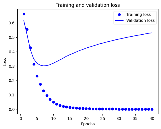
plt.title('Training and validation loss')
plt.xlabel('Epochs')
plt.ylabel('Loss')
plt.legend()
plt.show()
plt.clf()   # clear figure

plt.plot(epochs, acc, 'bo', label='Training acc')
plt.plot(epochs, val_acc, 'b', label='Validation acc')
plt.title('Training and validation accuracy')
plt.xlabel('Epochs')
plt.ylabel('Accuracy')
plt.legend()

plt.show()

Trong biểu đồ này, các dấu chấm thể hiện sự mất mát trong quá trình huấn luyện và độ chính xác, còn các đường liền là sự mất xác thực và độ chính xác.
Chú ý sự mất mát đào tạo giảm theo từng thời đại và tính chính xác đào tạo tăng lên theo từng thời đại. Điều này được mong đợi khi sử dụng tối ưu hóa giảm dần độ dốc — nó sẽ giảm thiểu số lượng mong muốn trên mỗi lần lặp.
Đây không phải là trường hợp của việc mất xác thực và độ chính xác — chúng dường như đạt đỉnh sau khoảng hai mươi kỷ nguyên. Đây là một ví dụ về overfitting: mô hình hoạt động tốt hơn trên dữ liệu đào tạo so với dữ liệu mà nó chưa từng thấy trước đây. Sau thời điểm này, mô hình quá tối ưu và nghe tin cơ quan đại diện cụ thể cho các dữ liệu huấn luyện mà không khái quát để kiểm tra dữ liệu.
Đối với trường hợp cụ thể này, chúng tôi có thể ngăn chặn việc trang bị quá mức bằng cách dừng đào tạo sau hai mươi kỷ nguyên hoặc lâu hơn. Sau đó, bạn sẽ thấy cách thực hiện việc này tự động với một cuộc gọi lại.
# MIT License
#
# Copyright (c) 2017 François Chollet
#
# Permission is hereby granted, free of charge, to any person obtaining a
# copy of this software and associated documentation files (the "Software"),
# to deal in the Software without restriction, including without limitation
# the rights to use, copy, modify, merge, publish, distribute, sublicense,
# and/or sell copies of the Software, and to permit persons to whom the
# Software is furnished to do so, subject to the following conditions:
#
# The above copyright notice and this permission notice shall be included in
# all copies or substantial portions of the Software.
#
# THE SOFTWARE IS PROVIDED "AS IS", WITHOUT WARRANTY OF ANY KIND, EXPRESS OR
# IMPLIED, INCLUDING BUT NOT LIMITED TO THE WARRANTIES OF MERCHANTABILITY,
# FITNESS FOR A PARTICULAR PURPOSE AND NONINFRINGEMENT. IN NO EVENT SHALL
# THE AUTHORS OR COPYRIGHT HOLDERS BE LIABLE FOR ANY CLAIM, DAMAGES OR OTHER
# LIABILITY, WHETHER IN AN ACTION OF CONTRACT, TORT OR OTHERWISE, ARISING
# FROM, OUT OF OR IN CONNECTION WITH THE SOFTWARE OR THE USE OR OTHER
# DEALINGS IN THE SOFTWARE.