Phân loại âm thanh với YAMNet

YAMNet là một mạng lưới sâu mà dự đoán 521 sự kiện âm thanh lớp học từ corpus AudioSet-YouTube nó được thí nghiệm trên. Nó sử dụng các Mobilenet_v1 kiến trúc chập depthwise-tách.

import tensorflow as tf
import tensorflow_hub as hub
import numpy as np
import csv

import matplotlib.pyplot as plt
from IPython.display import Audio
from scipy.io import wavfile

Tải Mô hình từ TensorFlow Hub.

Lưu ý: để đọc tài liệu chỉ cần làm theo các mô hình của url

# Load the model.
model = hub.load('https://tfhub.dev/google/yamnet/1')

Các tập tin nhãn sẽ được nạp từ các mô hình tài sản và có mặt tại model.class_map_path() . Bạn sẽ được tải nó trên class_names biến.

# Find the name of the class with the top score when mean-aggregated across frames.
def class_names_from_csv(class_map_csv_text):
  """Returns list of class names corresponding to score vector."""
  class_names = []
  with tf.io.gfile.GFile(class_map_csv_text) as csvfile:
    reader = csv.DictReader(csvfile)
    for row in reader:
      class_names.append(row['display_name'])

  return class_names

class_map_path = model.class_map_path().numpy()
class_names = class_names_from_csv(class_map_path)

Thêm một phương pháp để xác minh và chuyển đổi âm thanh đã tải về sample_rate (16K) thích hợp, nếu không nó sẽ ảnh hưởng đến kết quả của mô hình.

def ensure_sample_rate(original_sample_rate, waveform,
                       desired_sample_rate=16000):
  """Resample waveform if required."""
  if original_sample_rate != desired_sample_rate:
    desired_length = int(round(float(len(waveform)) /
                               original_sample_rate * desired_sample_rate))
    waveform = scipy.signal.resample(waveform, desired_length)
  return desired_sample_rate, waveform

Tải xuống và chuẩn bị tệp âm thanh

Tại đây, bạn sẽ tải xuống một tệp wav và nghe nó. Nếu bạn đã có sẵn một tập tin, chỉ cần tải nó lên colab và sử dụng nó thay thế.

Lưu ý: Các tập tin âm thanh sẽ phải là một tập tin wav mono ở tỷ lệ mẫu 16kHz.

curl -O https://storage.googleapis.com/audioset/speech_whistling2.wav

% Total    % Received % Xferd  Average Speed   Time    Time     Time  Current
                                 Dload  Upload   Total   Spent    Left  Speed
100  153k  100  153k    0     0   267k      0 --:--:-- --:--:-- --:--:--  266k

curl -O https://storage.googleapis.com/audioset/miaow_16k.wav

% Total    % Received % Xferd  Average Speed   Time    Time     Time  Current
                                 Dload  Upload   Total   Spent    Left  Speed
100  210k  100  210k    0     0   185k      0  0:00:01  0:00:01 --:--:--  185k

# wav_file_name = 'speech_whistling2.wav'
wav_file_name = 'miaow_16k.wav'
sample_rate, wav_data = wavfile.read(wav_file_name, 'rb')
sample_rate, wav_data = ensure_sample_rate(sample_rate, wav_data)

# Show some basic information about the audio.
duration = len(wav_data)/sample_rate
print(f'Sample rate: {sample_rate} Hz')
print(f'Total duration: {duration:.2f}s')
print(f'Size of the input: {len(wav_data)}')

# Listening to the wav file.
Audio(wav_data, rate=sample_rate)

Sample rate: 16000 Hz
Total duration: 6.73s
Size of the input: 107698
/tmpfs/src/tf_docs_env/lib/python3.7/site-packages/ipykernel_launcher.py:3: WavFileWarning: Chunk (non-data) not understood, skipping it.
  This is separate from the ipykernel package so we can avoid doing imports until

Các wav_data cần phải được bình thường đến các giá trị trong [-1.0, 1.0] (như đã nêu trong của mô hình tài liệu ).

waveform = wav_data / tf.int16.max

Thực thi mô hình

Bây giờ là phần dễ dàng: sử dụng dữ liệu đã được chuẩn bị sẵn, bạn chỉ cần gọi mô hình và nhận: điểm số, nhúng và biểu đồ quang phổ.

Điểm số là kết quả chính mà bạn sẽ sử dụng. Biểu đồ quang phổ bạn sẽ sử dụng để thực hiện một số hình dung sau này.

# Run the model, check the output.
scores, embeddings, spectrogram = model(waveform)

scores_np = scores.numpy()
spectrogram_np = spectrogram.numpy()
infered_class = class_names[scores_np.mean(axis=0).argmax()]
print(f'The main sound is: {infered_class}')

The main sound is: Animal

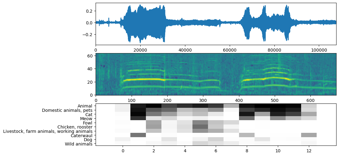
Hình dung

YAMNet cũng trả về một số thông tin bổ sung mà chúng tôi có thể sử dụng để hình dung. Chúng ta hãy xem xét Dạng sóng, biểu đồ quang phổ và các lớp hàng đầu được suy ra.

plt.figure(figsize=(10, 6))

# Plot the waveform.
plt.subplot(3, 1, 1)
plt.plot(waveform)
plt.xlim([0, len(waveform)])

# Plot the log-mel spectrogram (returned by the model).
plt.subplot(3, 1, 2)
plt.imshow(spectrogram_np.T, aspect='auto', interpolation='nearest', origin='lower')

# Plot and label the model output scores for the top-scoring classes.
mean_scores = np.mean(scores, axis=0)
top_n = 10
top_class_indices = np.argsort(mean_scores)[::-1][:top_n]
plt.subplot(3, 1, 3)
plt.imshow(scores_np[:, top_class_indices].T, aspect='auto', interpolation='nearest', cmap='gray_r')

# patch_padding = (PATCH_WINDOW_SECONDS / 2) / PATCH_HOP_SECONDS
# values from the model documentation
patch_padding = (0.025 / 2) / 0.01
plt.xlim([-patch_padding-0.5, scores.shape[0] + patch_padding-0.5])
# Label the top_N classes.
yticks = range(0, top_n, 1)
plt.yticks(yticks, [class_names[top_class_indices[x]] for x in yticks])
_ = plt.ylim(-0.5 + np.array([top_n, 0]))