Licensed under the MIT License
# Permission is hereby granted, free of charge, to any person obtaining a copy
# of this software and associated documentation files (the "Software"), to deal
# in the Software without restriction, including without limitation the rights
# to use, copy, modify, merge, publish, distribute, sublicense, and/or sell
# copies of the Software, and to permit persons to whom the Software is
# furnished to do so, subject to the following conditions:
#
# The above copyright notice and this permission notice shall be included in all
# copies or substantial portions of the Software.
#
# THE SOFTWARE IS PROVIDED "AS IS", WITHOUT WARRANTY OF ANY KIND, EXPRESS OR
# IMPLIED, INCLUDING BUT NOT LIMITED TO THE WARRANTIES OF MERCHANTABILITY,
# FITNESS FOR A PARTICULAR PURPOSE AND NONINFRINGEMENT. IN NO EVENT SHALL THE
# AUTHORS OR COPYRIGHT HOLDERS BE LIABLE FOR ANY CLAIM, DAMAGES OR OTHER
# LIABILITY, WHETHER IN AN ACTION OF CONTRACT, TORT OR OTHERWISE, ARISING FROM,
# OUT OF OR IN CONNECTION WITH THE SOFTWARE OR THE USE OR OTHER DEALINGS IN THE
# SOFTWARE.
| |
 在 Github 上查看源代码 在 Github 上查看源代码 |
|
2020 年初,为了减缓 COVID-19 的传播速度,欧洲各国采取了多种非药物干预措施(例如关闭非必要业务、隔离个别病例、禁止旅行等措施)鼓励民众保持社交距离。帝国理工学院 COVID-19 应急响应小组在其论文“Estimating the number of infections and the impact of non-pharmaceutical interventions on COVID-19 in 11 European countries”中,结合使用贝叶斯分层模型和机械式流行病学模型,分析了这些措施的有效性。
此 Colab 包含该分析的 TensorFlow Probability (TFP) 实现,结构如下:
- “模型设置”会定义疾病传播和由此导致死亡的流行病学模型、模型参数的贝叶斯先验分布,以及参数值条件下的死亡人数分布。
- “数据预处理”会加载关于每个国家/地区干预措施的时间与类型、随时间推移的死亡人数和估计感染者死亡率的数据。
- “模型推断”会构建贝叶斯分层模型并运行汉密尔顿蒙特卡洛 (HMC) 算法,对参数的后验分布进行采样。
- “结果”会显示相关数量(例如,预报的死亡人数,以及在没有干预措施的情况下的反事实死亡人数)的后验预测分布。
该论文发现有证据表明,各个国家/地区已设法减少了每个感染者传播的新感染人数 (\(R_t\)),但可信区间包含了 \(R_t=1\)(超过该值,流行病将继续蔓延),现在对干预措施的有效性得出强有力的结论还为时尚早。论文的 Stan 代码发布在作者的 Github 代码仓库中,此 Colab 复制的是版本 2。
pip3 install -q git+git://github.com/arviz-devs/arviz.gitpip3 install -q tf-nightly tfp-nightly
Imports
import collections
from pprint import pprint

import numpy as np
import pandas as pd

import matplotlib.pyplot as plt

%config InlineBackend.figure_format = 'retina'

import tensorflow.compat.v2 as tf
import tensorflow_probability as tfp
from tensorflow_probability.python.internal import prefer_static as ps

tf.enable_v2_behavior()

# Globally Enable XLA.
# tf.config.optimizer.set_jit(True)

try:
  physical_devices = tf.config.list_physical_devices('GPU')
  tf.config.experimental.set_memory_growth(physical_devices[0], True)
except:
  # Invalid device or cannot modify virtual devices once initialized.
  pass

tfb = tfp.bijectors
tfd = tfp.distributions

DTYPE = np.float32
1 模型设置
1.1 感染和死亡的机械模型
感染模型模拟每个国家/地区随时间推移的感染人数。输入数据是干预措施的时间与类型、人口规模和初始病例。参数控制干预措施的有效性和疾病传播率。预期死亡人数模型会对预测的感染应用死亡率。
感染模型会使用序列间隔分布(从成为感染者到感染其他人之间的天数分布)对先前的每日感染人数执行卷积。在每个时间步骤,时间 \(t\), \(n_t\) 处的新感染人数计算公式如下:
\begin{equation} \sum_{i=0}^{t-1} n_i \mu_t \text{p}(\text{被在} i \text{处感染的人感染} | t \text{处的新感染者})\end{equation} 其中 \(\mu_t=R_t\),条件概率存储在 conv_serial_interval 中,定义如下。
预期死亡人数模型会对每日感染人数以及感染与死亡之间的天数分布执行卷积。也就是说,\(t\) 日的预期死亡人数计算公式如下:
\begin{equation} \sum_{i=0}^{t-1} n_i\text{p(\(t\) 日死亡 | \(i\) 日感染)} \end{equation} 其中条件概率存储在 conv_fatality_rate 中,定义如下。
from tensorflow_probability.python.internal import broadcast_util as bu

def predict_infections(
    intervention_indicators, population, initial_cases, mu, alpha_hier,
    conv_serial_interval, initial_days, total_days):
  """Predict the number of infections by forward-simulation.

  Args:
    intervention_indicators: Binary array of shape
      `[num_countries, total_days, num_interventions]`, in which `1` indicates
      the intervention is active in that country at that time and `0` indicates
      otherwise.
    population: Vector of length `num_countries`. Population of each country.
    initial_cases: Array of shape `[batch_size, num_countries]`. Number of cases
      in each country at the start of the simulation.
    mu: Array of shape `[batch_size, num_countries]`. Initial reproduction rate
      (R_0) by country.
    alpha_hier: Array of shape `[batch_size, num_interventions]` representing
      the effectiveness of interventions.
    conv_serial_interval: Array of shape
      `[total_days - initial_days, total_days]` output from
      `make_conv_serial_interval`. Convolution kernel for serial interval
      distribution.
    initial_days: Integer, number of sequential days to seed infections after
      the 10th death in a country. (N0 in the authors' Stan code.)
    total_days: Integer, number of days of observed data plus days to forecast.
      (N2 in the authors' Stan code.)
  Returns:
    predicted_infections: Array of shape
      `[total_days, batch_size, num_countries]`. (Batched) predicted number of
      infections over time and by country.
  """
  alpha = alpha_hier - tf.cast(np.log(1.05) / 6.0, DTYPE)

  # Multiply the effectiveness of each intervention in each country (alpha)
  # by the indicator variable for whether the intervention was active and sum
  # over interventions, yielding an array of shape
  # [total_days, batch_size, num_countries] that represents the total effectiveness of
  # all interventions in each country on each day (for a batch of data).
  linear_prediction = tf.einsum(
      'ijk,...k->j...i', intervention_indicators, alpha)

  # Adjust the reproduction rate per country downward, according to the
  # effectiveness of the interventions.
  rt = mu * tf.exp(-linear_prediction, name='reproduction_rate')

  # Initialize storage array for daily infections and seed it with initial
  # cases.
  daily_infections = tf.TensorArray(
      dtype=DTYPE, size=total_days, element_shape=initial_cases.shape)
  for i in range(initial_days):
    daily_infections = daily_infections.write(i, initial_cases)

  # Initialize cumulative cases.
  init_cumulative_infections = initial_cases * initial_days

  # Simulate forward for total_days days.
  cond = lambda i, *_: i < total_days
  def body(i, prev_daily_infections, prev_cumulative_infections):
    # The probability distribution over days j that someone infected on day i
    # caught the virus from someone infected on day j.
    p_infected_on_day = tf.gather(
        conv_serial_interval, i - initial_days, axis=0)

    # Multiply p_infected_on_day by the number previous infections each day and
    # by mu, and sum to obtain new infections on day i. Mu is adjusted by
    # the fraction of the population already infected, so that the population
    # size is the upper limit on the number of infections.
    prev_daily_infections_array = prev_daily_infections.stack()
    to_sum = prev_daily_infections_array * bu.left_justified_expand_dims_like(
        p_infected_on_day, prev_daily_infections_array)
    convolution = tf.reduce_sum(to_sum, axis=0)
    rt_adj = (
        (population - prev_cumulative_infections) / population
        ) * tf.gather(rt, i)
    new_infections = rt_adj * convolution

    # Update the prediction array and the cumulative number of infections.
    daily_infections = prev_daily_infections.write(i, new_infections)
    cumulative_infections = prev_cumulative_infections + new_infections
    return i + 1, daily_infections, cumulative_infections

  _, daily_infections_final, last_cumm_sum = tf.while_loop(
      cond, body,
      (initial_days, daily_infections, init_cumulative_infections),
      maximum_iterations=(total_days - initial_days))
  return daily_infections_final.stack()

def predict_deaths(predicted_infections, ifr_noise, conv_fatality_rate):
  """Expected number of reported deaths by country, by day.

  Args:
    predicted_infections: Array of shape
      `[total_days, batch_size, num_countries]` output from
      `predict_infections`.
    ifr_noise: Array of shape `[batch_size, num_countries]`. Noise in Infection
      Fatality Rate (IFR).
    conv_fatality_rate: Array of shape
      `[total_days - 1, total_days, num_countries]`. Convolutional kernel for
      calculating fatalities, output from `make_conv_fatality_rate`.
  Returns:
    predicted_deaths: Array of shape `[total_days, batch_size, num_countries]`.
      (Batched) predicted number of deaths over time and by country.
  """
  # Multiply the number of infections on day j by the probability of death
  # on day i given infection on day j, and sum over j. This yields the expected
  result_remainder = tf.einsum(
      'i...j,kij->k...j', predicted_infections, conv_fatality_rate) * ifr_noise

  # Concatenate the result with a vector of zeros so that the first day is
  # included.
  result_temp = 1e-15 * predicted_infections[:1]
  return tf.concat([result_temp, result_remainder], axis=0)
1.2 参数值的先验
在这里,我们定义模型参数的联合先验分布。许多参数值被假定独立,因此先验可表示为:
\(\text p(\tau, y, \psi, \kappa, \mu, \alpha) = \text p(\tau)\text p(y|\tau)\text p(\psi)\text p(\kappa)\text p(\mu|\kappa)\text p(\alpha)\text p(\epsilon)\)
其中:
- \(\tau\) 是每个国家/地区初始病例数 (\(y = y_1, ... y_{\text{num_countries} }\)) 的指数分布的共享率参数。
- \(\psi\) 是死亡人数负二项分布中的参数。
- \(\kappa\) 是每个国家/地区初始再生数(\(\mu = \mu_1, ..., \mu_{\text{num_countries} }\),表示每个感染者传播的二代病例数)的半正态分布的共享尺度参数。
- \(\alpha = \alpha_1, ..., \alpha_6\) 是六项干预措施中每一项的有效性。
- \(\epsilon\)(在代码中调用了
ifr_noise,在作者的 Stan 代码之后)是感染死亡率 (IFR) 中的噪声。
我们将此模型表示为 TFP JointDistribution,这是一种 TFP 分布,可以表达概率图模型。
def make_jd_prior(num_countries, num_interventions):
  return tfd.JointDistributionSequentialAutoBatched([
      # Rate parameter for the distribution of initial cases (tau).
      tfd.Exponential(rate=tf.cast(0.03, DTYPE)),

      # Initial cases for each country.
      lambda tau: tfd.Sample(
          tfd.Exponential(rate=tf.cast(1, DTYPE) / tau),
          sample_shape=num_countries),

      # Parameter in Negative Binomial model for deaths (psi).
      tfd.HalfNormal(scale=tf.cast(5, DTYPE)),

      # Parameter in the distribution over the initial reproduction number, R_0
      # (kappa).
      tfd.HalfNormal(scale=tf.cast(0.5, DTYPE)),

      # Initial reproduction number, R_0, for each country (mu).
      lambda kappa: tfd.Sample(
          tfd.TruncatedNormal(loc=3.28, scale=kappa, low=1e-5, high=1e5),
          sample_shape=num_countries),

      # Impact of interventions (alpha; shared for all countries).
      tfd.Sample(
          tfd.Gamma(tf.cast(0.1667, DTYPE), 1), sample_shape=num_interventions),

      # Multiplicative noise in Infection Fatality Rate.
      tfd.Sample(
          tfd.TruncatedNormal(
              loc=tf.cast(1., DTYPE), scale=0.1, low=1e-5, high=1e5),
              sample_shape=num_countries)
  ])
1.3 以参数值为条件的观测死亡人数的似然
似然模型表达 \(p(\text{死亡人数} | \tau, y, \psi, \kappa, \mu, \alpha, \epsilon)\)。它以参数为条件将模型应用于感染人数和预期死亡人数,并假设实际死亡人数遵循负二项分布。
def make_likelihood_fn(
    intervention_indicators, population, deaths,
    infection_fatality_rate, initial_days, total_days):

  # Create a mask for the initial days of simulated data, as they are not
  # counted in the likelihood.
  observed_deaths = tf.constant(deaths.T[np.newaxis, ...], dtype=DTYPE)
  mask_temp = deaths != -1
  mask_temp[:, :START_DAYS] = False
  observed_deaths_mask = tf.constant(mask_temp.T[np.newaxis, ...])

  conv_serial_interval = make_conv_serial_interval(initial_days, total_days)
  conv_fatality_rate = make_conv_fatality_rate(
      infection_fatality_rate, total_days)

  def likelihood_fn(tau, initial_cases, psi, kappa, mu, alpha_hier, ifr_noise):
    # Run models for infections and expected deaths
    predicted_infections = predict_infections(
        intervention_indicators, population, initial_cases, mu, alpha_hier,
        conv_serial_interval, initial_days, total_days)
    e_deaths_all_countries = predict_deaths(
        predicted_infections, ifr_noise, conv_fatality_rate)

    # Construct the Negative Binomial distribution for deaths by country.
    mu_m = tf.transpose(e_deaths_all_countries, [1, 0, 2])
    psi_m = psi[..., tf.newaxis, tf.newaxis]
    probs = tf.clip_by_value(mu_m / (mu_m + psi_m), 1e-9, 1.)
    likelihood_elementwise = tfd.NegativeBinomial(
        total_count=psi_m, probs=probs).log_prob(observed_deaths)
    return tf.reduce_sum(
        tf.where(observed_deaths_mask,
                likelihood_elementwise,
                tf.zeros_like(likelihood_elementwise)),
        axis=[-2, -1])

  return likelihood_fn
1.4 感染后的死亡概率
本部分计算感染后几天的死亡人数分布。它假设从感染到死亡的时间是两个 Gamma 变量之和,分别代表从感染到发病的时间和从发病到死亡的时间。将死亡时间分布与 Verity 等人(2020 年)论文中的感染死亡率相结合,计算感染后几天的死亡概率。
def daily_fatality_probability(infection_fatality_rate, total_days):
  """Computes the probability of death `d` days after infection."""

  # Convert from alternative Gamma parametrization and construct distributions
  # for number of days from infection to onset and onset to death.
  concentration1 = tf.cast((1. / 0.86)**2, DTYPE)
  rate1 = concentration1 / 5.1
  concentration2 = tf.cast((1. / 0.45)**2, DTYPE)
  rate2 = concentration2 / 18.8
  infection_to_onset = tfd.Gamma(concentration=concentration1, rate=rate1)
  onset_to_death = tfd.Gamma(concentration=concentration2, rate=rate2)

  # Create empirical distribution for number of days from infection to death.
  inf_to_death_dist = tfd.Empirical(
      infection_to_onset.sample([5e6]) + onset_to_death.sample([5e6]))

  # Subtract the CDF value at day i from the value at day i + 1 to compute the
  # probability of death on day i given infection on day 0, and given that
  # death (not recovery) is the outcome.
  times = np.arange(total_days + 1., dtype=DTYPE) + 0.5
  cdf = inf_to_death_dist.cdf(times).numpy()
  f_before_ifr = cdf[1:] - cdf[:-1]
  # Explicitly set the zeroth value to the empirical cdf at time 1.5, to include
  # the mass between time 0 and time .5.
  f_before_ifr[0] = cdf[1]

  # Multiply the daily fatality rates conditional on infection and eventual
  # death (f_before_ifr) by the infection fatality rates (probability of death
  # given intection) to obtain the probability of death on day i conditional
  # on infection on day 0.
  return infection_fatality_rate[..., np.newaxis] * f_before_ifr

def make_conv_fatality_rate(infection_fatality_rate, total_days):
  """Computes the probability of death on day `i` given infection on day `j`."""
  p_fatal_all_countries = daily_fatality_probability(
      infection_fatality_rate, total_days)

  # Use the probability of death d days after infection in each country
  # to build an array of shape [total_days - 1, total_days, num_countries],
  # where the element [i, j, c] is the probability of death on day i+1 given
  # infection on day j in country c.
  conv_fatality_rate = np.zeros(
      [total_days - 1, total_days, p_fatal_all_countries.shape[0]])
  for n in range(1, total_days):
    conv_fatality_rate[n - 1, 0:n, :] = (
        p_fatal_all_countries[:, n - 1::-1]).T
  return tf.constant(conv_fatality_rate, dtype=DTYPE)
1.5 序列间隔
序列间隔是疾病传播链中连续病例之间的时间,假设遵循 Gamma 分布。我们使用序列间隔分布计算 \(i\) 日感染的人从先前在 \(j\) 日感染的人身上感染病毒的概率(conv_serial_interval 参数到 predict_infections)。
def make_conv_serial_interval(initial_days, total_days):
  """Construct the convolutional kernel for infection timing."""

  g = tfd.Gamma(tf.cast(1. / (0.62**2), DTYPE), 1./(6.5*0.62**2))
  g_cdf = g.cdf(np.arange(total_days, dtype=DTYPE))

  # Approximate the probability mass function for the number of days between
  # successive infections.
  serial_interval = g_cdf[1:] - g_cdf[:-1]

  # `conv_serial_interval` is an array of shape
  # [total_days - initial_days, total_days] in which entry [i, j] contains the
  # probability that an individual infected on day i + initial_days caught the
  # virus from someone infected on day j.
  conv_serial_interval = np.zeros([total_days - initial_days, total_days])
  for n in range(initial_days, total_days):
    conv_serial_interval[n - initial_days, 0:n] = serial_interval[n - 1::-1]
  return tf.constant(conv_serial_interval, dtype=DTYPE)
2 数据预处理
COUNTRIES = [
    'Austria',
    'Belgium',
    'Denmark',
    'France',
    'Germany',
    'Italy',
    'Norway',
    'Spain',
    'Sweden',
    'Switzerland',
    'United_Kingdom'
]
2.1 Fetch and preprocess interventions data
raw_interventions = pd.read_csv(
    'https://raw.githubusercontent.com/ImperialCollegeLondon/covid19model/master/data/interventions.csv')

raw_interventions['Date effective'] = pd.to_datetime(
    raw_interventions['Date effective'], dayfirst=True)
interventions = raw_interventions.pivot(index='Country', columns='Type', values='Date effective')

# If any interventions happened after the lockdown, use the date of the lockdown.
for col in interventions.columns:
  idx = interventions[col] > interventions['Lockdown']
  interventions.loc[idx, col] = interventions[idx]['Lockdown']

num_countries = len(COUNTRIES)
2.2 Fetch case/death data and join to interventions
# Load the case data
data = pd.read_csv('https://raw.githubusercontent.com/ImperialCollegeLondon/covid19model/master/data/COVID-19-up-to-date.csv')
# You can also use the dataset directly from european cdc (where the ICL model fetch their data from)
# data = pd.read_csv('https://opendata.ecdc.europa.eu/covid19/casedistribution/csv')

data['country'] = data['countriesAndTerritories']
data = data[['dateRep', 'cases', 'deaths', 'country']]
data = data[data['country'].isin(COUNTRIES)]
data['dateRep'] = pd.to_datetime(data['dateRep'], format='%d/%m/%Y')

# Add 0/1 features for whether or not each intevention was in place.
data = data.join(interventions, on='country', how='outer')
for col in interventions.columns:
  data[col] = (data['dateRep'] >= data[col]).astype(int)

# Add "any_intevention" 0/1 feature.
any_intervention_list = ['Schools + Universities',
                         'Self-isolating if ill',
                         'Public events',
                         'Lockdown',
                         'Social distancing encouraged']
data['any_intervention'] = (
    data[any_intervention_list].apply(np.sum, 'columns') > 0).astype(int)

# Index by country and date.
data = data.sort_values(by=['country', 'dateRep'])
data = data.set_index(['country', 'dateRep'])
2.3 Fetch and process Infected Fatality Ratio and population data
infected_fatality_ratio = pd.read_csv(
    'https://raw.githubusercontent.com/ImperialCollegeLondon/covid19model/master/data/popt_ifr.csv')

infected_fatality_ratio = infected_fatality_ratio.replace(to_replace='United Kingdom', value='United_Kingdom')
infected_fatality_ratio['Country'] = infected_fatality_ratio.iloc[:, 1]
infected_fatality_ratio = infected_fatality_ratio[infected_fatality_ratio['Country'].isin(COUNTRIES)]
infected_fatality_ratio = infected_fatality_ratio[
  ['Country', 'popt', 'ifr']].set_index('Country')
infected_fatality_ratio = infected_fatality_ratio.sort_index()
infection_fatality_rate = infected_fatality_ratio['ifr'].to_numpy()
population_value = infected_fatality_ratio['popt'].to_numpy()
2.4 预处理特定于国家/地区的数据
# Model up to 75 days of data for each country, starting 30 days before the
# tenth cumulative death.
START_DAYS = 30
MAX_DAYS = 102
COVARIATE_COLUMNS = any_intervention_list + ['any_intervention']

# Initialize an array for number of deaths.
deaths = -np.ones((num_countries, MAX_DAYS), dtype=DTYPE)

# Assuming every intervention is still inplace in the unobserved future
num_interventions = len(COVARIATE_COLUMNS)
intervention_indicators = np.ones((num_countries, MAX_DAYS, num_interventions))

first_days = {}
for i, c in enumerate(COUNTRIES):
  c_data = data.loc[c]

  # Include data only after 10th death in a country.
  mask = c_data['deaths'].cumsum() >= 10

  # Get the date that the epidemic starts in a country.
  first_day = c_data.index[mask][0] - pd.to_timedelta(START_DAYS, 'days')
  c_data = c_data.truncate(before=first_day)

  # Truncate the data after 28 March 2020 for comparison with Flaxman et al.
  c_data = c_data.truncate(after='2020-03-28')

  c_data = c_data.iloc[:MAX_DAYS]
  days_of_data = c_data.shape[0]
  deaths[i, :days_of_data] = c_data['deaths']
  intervention_indicators[i, :days_of_data] = c_data[
    COVARIATE_COLUMNS].to_numpy()
  first_days[c] = first_day

# Number of sequential days to seed infections after the 10th death in a
# country. (N0 in authors' Stan code.)
INITIAL_DAYS = 6

# Number of days of observed data plus days to forecast. (N2 in authors' Stan
# code.)
TOTAL_DAYS = deaths.shape[1]
3 模型推断
Flaxman 等人 (2020) 使用 Stan 通过汉密尔顿蒙特卡洛 (HMC) 和 No-U-Turn Sampler (NUTS) 从参数后验中采样。
在这里,我们应用具有对偶平均步长适应的 HMC。我们使用 HMC 的试运行来进行预处理和初始化。
推断会在几分钟内在 GPU 上运行。
3.1 构建模型的先验和似然
jd_prior = make_jd_prior(num_countries, num_interventions)
likelihood_fn = make_likelihood_fn(
    intervention_indicators, population_value, deaths,
    infection_fatality_rate, INITIAL_DAYS, TOTAL_DAYS)
3.2 效用函数
def get_bijectors_from_samples(samples, unconstraining_bijectors, batch_axes):
  """Fit bijectors to the samples of a distribution.

  This fits a diagonal covariance multivariate Gaussian transformed by the
  `unconstraining_bijectors` to the provided samples. The resultant
  transformation can be used to precondition MCMC and other inference methods.
  """
  state_std = [
      tf.math.reduce_std(bij.inverse(x), axis=batch_axes)
      for x, bij in zip(samples, unconstraining_bijectors)
  ]
  state_mu = [
      tf.math.reduce_mean(bij.inverse(x), axis=batch_axes)
      for x, bij in zip(samples, unconstraining_bijectors)
  ]
  return [tfb.Chain([cb, tfb.Shift(sh), tfb.Scale(sc)])
          for cb, sh, sc in zip(unconstraining_bijectors, state_mu, state_std)]

def generate_init_state_and_bijectors_from_prior(nchain, unconstraining_bijectors):
  """Creates an initial MCMC state, and bijectors from the prior."""
  prior_samples = jd_prior.sample(4096)

  bijectors = get_bijectors_from_samples(
      prior_samples, unconstraining_bijectors, batch_axes=0)

  init_state = [
    bij(tf.zeros([nchain] + list(s), DTYPE))
    for s, bij in zip(jd_prior.event_shape, bijectors)
  ]

  return init_state, bijectors
@tf.function(autograph=False, experimental_compile=True)
def sample_hmc(
    init_state,
    step_size,
    target_log_prob_fn,
    unconstraining_bijectors,
    num_steps=500,
    burnin=50,
    num_leapfrog_steps=10):

    def trace_fn(_, pkr):
        return {
            'target_log_prob': pkr.inner_results.inner_results.accepted_results.target_log_prob,
            'diverging': ~(pkr.inner_results.inner_results.log_accept_ratio > -1000.),
            'is_accepted': pkr.inner_results.inner_results.is_accepted,
            'step_size': [tf.exp(s) for s in pkr.log_averaging_step],
        }

    hmc = tfp.mcmc.HamiltonianMonteCarlo(
        target_log_prob_fn,
        step_size=step_size,
        num_leapfrog_steps=num_leapfrog_steps)

    hmc = tfp.mcmc.TransformedTransitionKernel(
        inner_kernel=hmc,
        bijector=unconstraining_bijectors)

    hmc = tfp.mcmc.DualAveragingStepSizeAdaptation(
        hmc,
        num_adaptation_steps=int(burnin * 0.8),
        target_accept_prob=0.8,
        decay_rate=0.5)

    # Sampling from the chain.
    return tfp.mcmc.sample_chain(
        num_results=burnin + num_steps,
        current_state=init_state,
        kernel=hmc,
        trace_fn=trace_fn)
3.3 定义事件空间双射器
从各向同性多元高斯分布进行采样时,HMC 的效率最高(Mangoubi 和 Smith (2017)),因此,第一步是将目标密度预处理为尽可能像该分布。
首先,我们将受约束的(例如,非负)变量转换为 HMC 所需的无约束空间。此外,我们使用 SinhArcsinh 双射器来控制转换后的目标密度的尾部重量;我们希望它们大致以 \(e^{-x^2}\) 下降。
unconstraining_bijectors = [
    tfb.Chain([tfb.Scale(tf.constant(1 / 0.03, DTYPE)), tfb.Softplus(),
                tfb.SinhArcsinh(tailweight=tf.constant(1.85, DTYPE))]), # tau
    tfb.Chain([tfb.Scale(tf.constant(1 / 0.03, DTYPE)), tfb.Softplus(),
                tfb.SinhArcsinh(tailweight=tf.constant(1.85, DTYPE))]), # initial_cases
    tfb.Softplus(), # psi
    tfb.Softplus(), # kappa
    tfb.Softplus(), # mu
    tfb.Chain([tfb.Scale(tf.constant(0.4, DTYPE)), tfb.Softplus(),
                tfb.SinhArcsinh(skewness=tf.constant(-0.2, DTYPE), tailweight=tf.constant(2., DTYPE))]), # alpha
    tfb.Softplus(), # ifr_noise
]
3.4 HMC 试运行
我们首先运行由先验预处理的 HMC ,在转换后的空间中从 0 初始化。我们不使用先验样本来初始化链,因为在实践中,由于那些样本数值不佳,往往会导致卡链。
%%time

nchain = 32

target_log_prob_fn = lambda *x: jd_prior.log_prob(*x) + likelihood_fn(*x)
init_state, bijectors = generate_init_state_and_bijectors_from_prior(nchain, unconstraining_bijectors)

# Each chain gets its own step size.
step_size = [tf.fill([nchain] + [1] * (len(s.shape) - 1), tf.constant(0.01, DTYPE)) for s in init_state]

burnin = 200
num_steps = 100

pilot_samples, pilot_sampler_stat = sample_hmc(
    init_state,
    step_size,
    target_log_prob_fn,
    bijectors,
    num_steps=num_steps,
    burnin=burnin,
    num_leapfrog_steps=10)
CPU times: user 56.8 s, sys: 2.34 s, total: 59.1 s
Wall time: 1min 1s
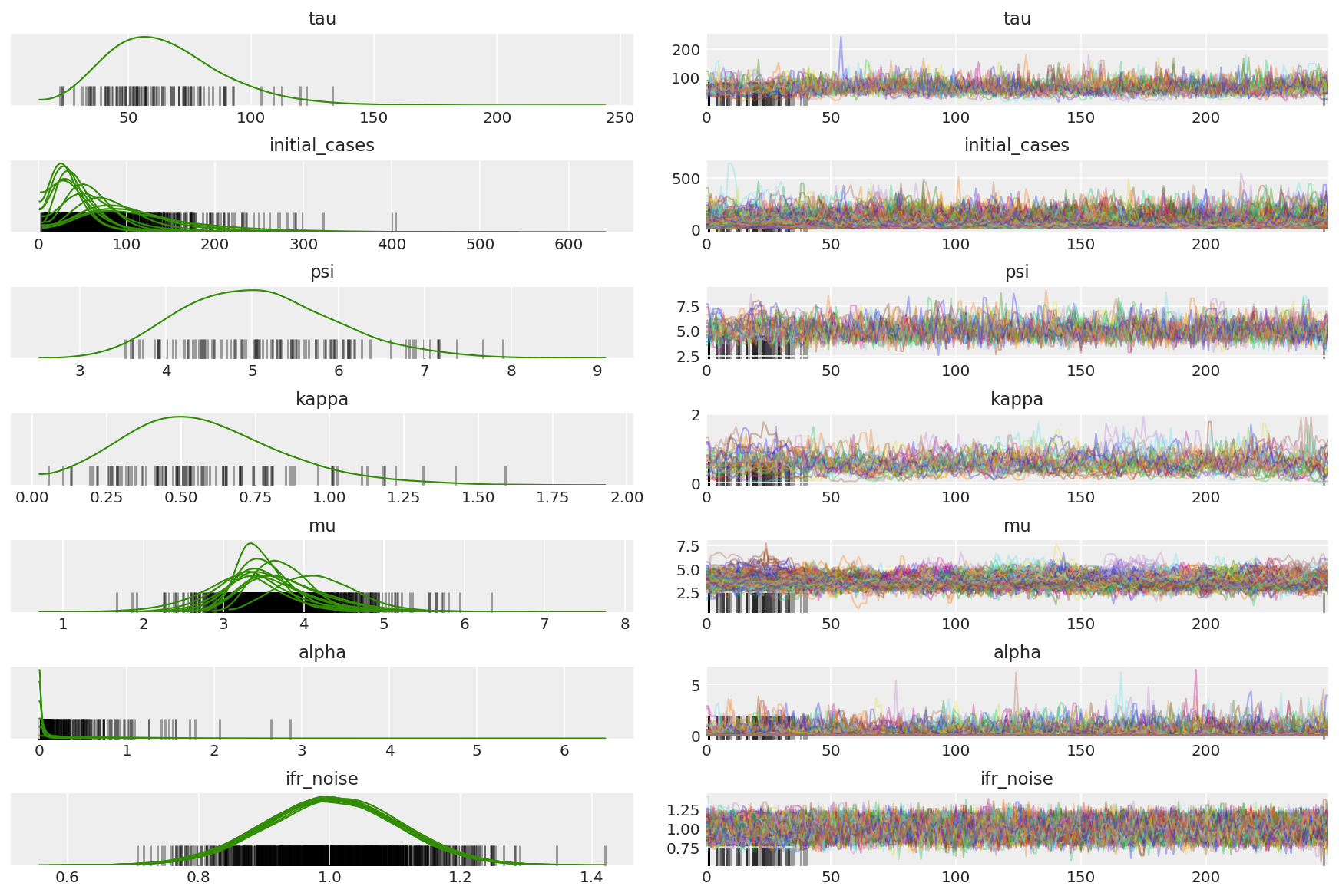
3.5 呈现试点样本
我们要寻找卡链并观察收敛情况。我们可以在这里进行正式诊断,但由于只是试运行,并不十分必要。
import arviz as az
az.style.use('arviz-darkgrid')
var_name = ['tau', 'initial_cases', 'psi', 'kappa', 'mu', 'alpha', 'ifr_noise']

pilot_with_warmup = {k: np.swapaxes(v.numpy(), 1, 0)
                     for k, v in zip(var_name, pilot_samples)}
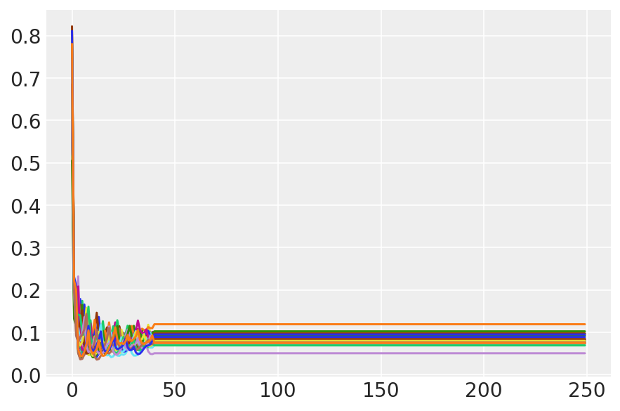
我们会在预热期间观察到差异,主要是因为对偶平均步长适应使用非常积极的搜索来寻找最佳步长。一旦适应关闭,差异也将消失。
az_trace = az.from_dict(posterior=pilot_with_warmup,
                        sample_stats={'diverging': np.swapaxes(pilot_sampler_stat['diverging'].numpy(), 0, 1)})
az.plot_trace(az_trace, combined=True, compact=True, figsize=(12, 8));
plt.plot(pilot_sampler_stat['step_size'][0]);
3.6 运行 HMC
原则上,我们可以使用试点样本进行最终分析(如果我们运行更长的时间以获得收敛),但是开始另一个 HMC 运行会更有效率,这次由试点样本进行预处理和初始化。
%%time

burnin = 50
num_steps = 200

bijectors = get_bijectors_from_samples([s[burnin:] for s in pilot_samples],
                                       unconstraining_bijectors=unconstraining_bijectors,
                                       batch_axes=(0, 1))

samples, sampler_stat = sample_hmc(
    [s[-1] for s in pilot_samples],
    [s[-1] for s in pilot_sampler_stat['step_size']],
    target_log_prob_fn,
    bijectors,
    num_steps=num_steps,
    burnin=burnin,
    num_leapfrog_steps=20)
CPU times: user 1min 26s, sys: 3.88 s, total: 1min 30s
Wall time: 1min 32s
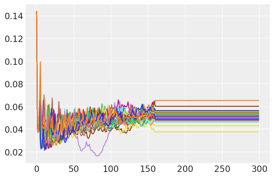
plt.plot(sampler_stat['step_size'][0]);
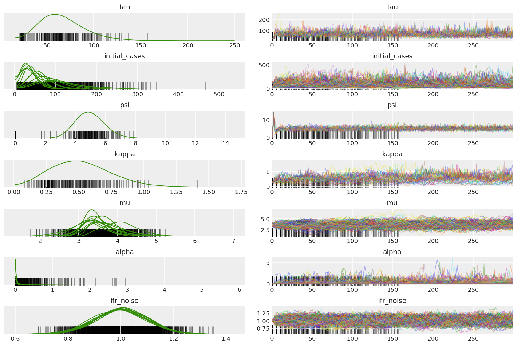
3.7 呈现样本
import arviz as az
az.style.use('arviz-darkgrid')
var_name = ['tau', 'initial_cases', 'psi', 'kappa', 'mu', 'alpha', 'ifr_noise']

posterior = {k: np.swapaxes(v.numpy()[burnin:], 1, 0)
             for k, v in zip(var_name, samples)}
posterior_with_warmup = {k: np.swapaxes(v.numpy(), 1, 0)
             for k, v in zip(var_name, samples)}
计算链的摘要。我们要找的是较高的 ESS 和接近 1 的 r_hat。
az.summary(posterior)
az_trace = az.from_dict(posterior=posterior_with_warmup,
                        sample_stats={'diverging': np.swapaxes(sampler_stat['diverging'].numpy(), 0, 1)})
az.plot_trace(az_trace, combined=True, compact=True, figsize=(12, 8));
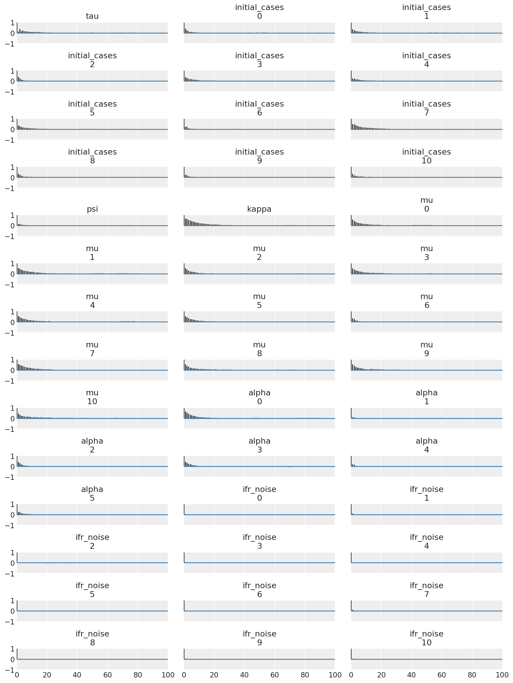
查看所有维度上的自相关函数很有意义。我们要找的是快速下降的函数,但又不至于下降到负值(这表明 HMC 发生共振,不利于遍历性,并且可能会引入偏差)。
with az.rc_context(rc={'plot.max_subplots': None}):
  az.plot_autocorr(posterior, combined=True, figsize=(12, 16), textsize=12);
4 结果
以下图表分析了 \(R_t\) 的后验预测分布、死亡人数和感染人数,类似于 Flaxman 等人(2020 年)论文的分析。
total_num_samples = np.prod(posterior['mu'].shape[:2])

# Calculate R_t given parameter estimates.
def rt_samples_batched(mu, intervention_indicators, alpha):
  linear_prediction = tf.reduce_sum(
      intervention_indicators * alpha[..., np.newaxis, np.newaxis, :], axis=-1)
  rt_hat = mu[..., tf.newaxis] * tf.exp(-linear_prediction, name='rt')
  return rt_hat

alpha_hat = tf.convert_to_tensor(
    posterior['alpha'].reshape(total_num_samples, posterior['alpha'].shape[-1]))
mu_hat = tf.convert_to_tensor(
    posterior['mu'].reshape(total_num_samples, num_countries))
rt_hat = rt_samples_batched(mu_hat, intervention_indicators, alpha_hat)
sampled_initial_cases = posterior['initial_cases'].reshape(
    total_num_samples, num_countries)
sampled_ifr_noise = posterior['ifr_noise'].reshape(
    total_num_samples, num_countries)
psi_hat = posterior['psi'].reshape([total_num_samples])

conv_serial_interval = make_conv_serial_interval(INITIAL_DAYS, TOTAL_DAYS)
conv_fatality_rate = make_conv_fatality_rate(infection_fatality_rate, TOTAL_DAYS)
pred_hat = predict_infections(
    intervention_indicators, population_value, sampled_initial_cases, mu_hat,
    alpha_hat, conv_serial_interval, INITIAL_DAYS, TOTAL_DAYS)
expected_deaths = predict_deaths(pred_hat, sampled_ifr_noise, conv_fatality_rate)

psi_m = psi_hat[np.newaxis, ..., np.newaxis]
probs = tf.clip_by_value(expected_deaths / (expected_deaths + psi_m), 1e-9, 1.)
predicted_deaths = tfd.NegativeBinomial(
    total_count=psi_m, probs=probs).sample()
# Predict counterfactual infections/deaths in the absence of interventions
no_intervention_infections = predict_infections(
    intervention_indicators,
    population_value,
    sampled_initial_cases,
    mu_hat,
    tf.zeros_like(alpha_hat),
    conv_serial_interval,
    INITIAL_DAYS, TOTAL_DAYS)

no_intervention_expected_deaths = predict_deaths(
    no_intervention_infections, sampled_ifr_noise, conv_fatality_rate)
probs = tf.clip_by_value(
    no_intervention_expected_deaths / (no_intervention_expected_deaths + psi_m),
    1e-9, 1.)
no_intervention_predicted_deaths = tfd.NegativeBinomial(
    total_count=psi_m, probs=probs).sample()
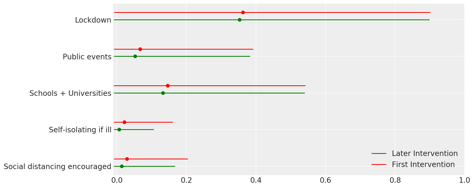
4.1 干预措施的有效性
与 Flaxman 等人(2020 年)论文中的图 4 类似。
def intervention_effectiveness(alpha):

  alpha_adj = 1. - np.exp(-alpha + np.log(1.05) / 6.)
  alpha_adj_first = (
      1. - np.exp(-alpha - alpha[..., -1:] + np.log(1.05) / 6.))

  fig, ax = plt.subplots(1, 1, figsize=[12, 6])
  intervention_perm = [2, 1, 3, 4, 0]
  percentile_vals = [2.5, 97.5]
  jitter = .2

  for ind in range(5):
    first_low, first_high = tfp.stats.percentile(
        alpha_adj_first[..., ind], percentile_vals)
    low, high = tfp.stats.percentile(
        alpha_adj[..., ind], percentile_vals)

    p_ind = intervention_perm[ind]
    ax.hlines(p_ind, low, high, label='Later Intervention', colors='g')
    ax.scatter(alpha_adj[..., ind].mean(), p_ind, color='g')
    ax.hlines(p_ind + jitter, first_low, first_high,
              label='First Intervention', colors='r')
    ax.scatter(alpha_adj_first[..., ind].mean(), p_ind + jitter, color='r')

    if ind == 0:
      plt.legend(loc='lower right')
  ax.set_yticks(range(5))
  ax.set_yticklabels(
      [any_intervention_list[intervention_perm.index(p)] for p in range(5)])
  ax.set_xlim([-0.01, 1.])
  r = fig.patch
  r.set_facecolor('white')

intervention_effectiveness(alpha_hat)
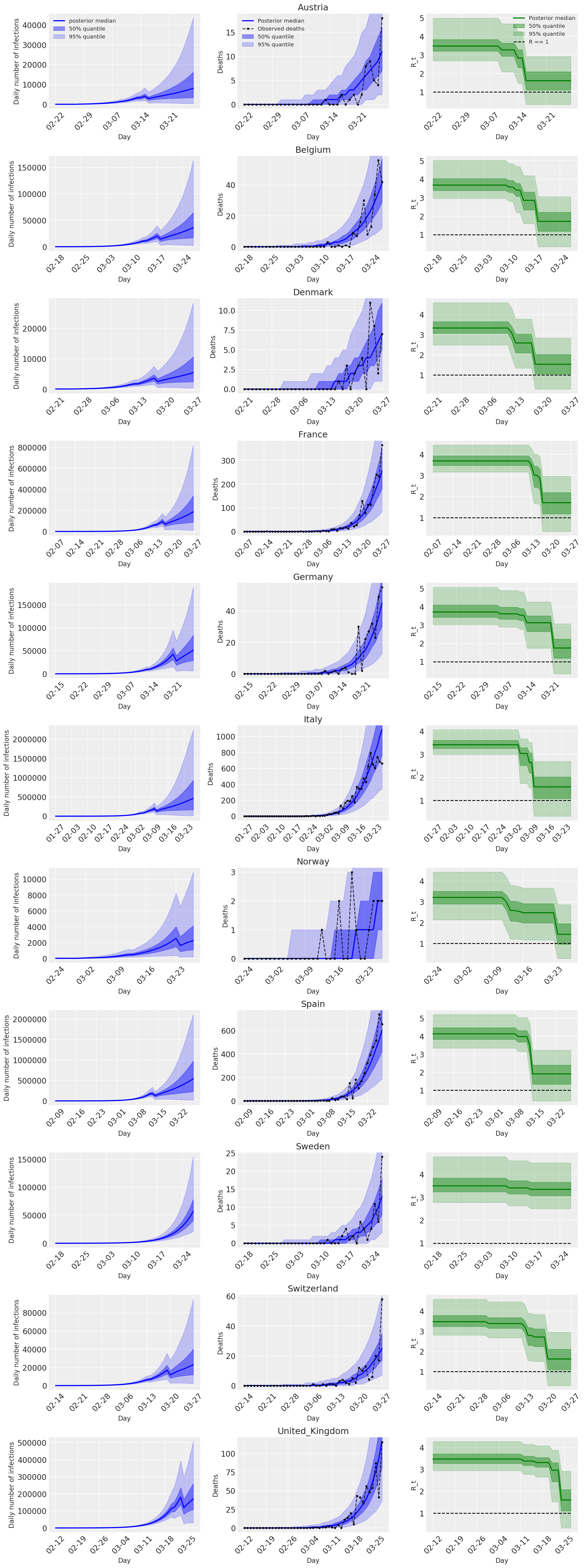
4.2 按国家/地区分列的感染人数、死亡人数和 R_t
与 Flaxman 等人(2020 年)论文中的图 2 类似。
import matplotlib.dates as mdates

plot_quantile = True
forecast_days = 0

fig, ax = plt.subplots(11, 3, figsize=(15, 40))

for ind, country in enumerate(COUNTRIES):
  num_days = (pd.to_datetime('2020-03-28') - first_days[country]).days + forecast_days
  dates = [(first_days[country] + i*pd.to_timedelta(1, 'days')).strftime('%m-%d') for i in range(num_days)]
  plot_dates = [dates[i] for i in range(0, num_days, 7)]

  # Plot daily number of infections
  infections = pred_hat[:, :, ind]
  posterior_quantile = np.percentile(infections, [2.5, 25, 50, 75, 97.5], axis=-1)
  ax[ind, 0].plot(
      dates, posterior_quantile[2, :num_days],
      color='b', label='posterior median', lw=2)
  if plot_quantile:
    ax[ind, 0].fill_between(
        dates, posterior_quantile[1, :num_days], posterior_quantile[3, :num_days],
        color='b', label='50% quantile', alpha=.4)
    ax[ind, 0].fill_between(
        dates, posterior_quantile[0, :num_days], posterior_quantile[4, :num_days],
        color='b', label='95% quantile', alpha=.2)

  ax[ind, 0].set_xticks(plot_dates)
  ax[ind, 0].xaxis.set_tick_params(rotation=45)
  ax[ind, 0].set_ylabel('Daily number of infections', fontsize='large')
  ax[ind, 0].set_xlabel('Day', fontsize='large')

  # Plot deaths
  ax[ind, 1].set_title(country)

  samples = predicted_deaths[:, :, ind]
  posterior_quantile = np.percentile(samples, [2.5, 25, 50, 75, 97.5], axis=-1)
  ax[ind, 1].plot(
      range(num_days), posterior_quantile[2, :num_days],
      color='b', label='Posterior median', lw=2)
  if plot_quantile:
    ax[ind, 1].fill_between(
        range(num_days), posterior_quantile[1, :num_days], posterior_quantile[3, :num_days],
        color='b', label='50% quantile', alpha=.4)
    ax[ind, 1].fill_between(
        range(num_days), posterior_quantile[0, :num_days], posterior_quantile[4, :num_days],
        color='b', label='95% quantile', alpha=.2)

  observed = deaths[ind, :]
  observed[observed == -1] = np.nan
  ax[ind, 1].plot(
      dates, observed[:num_days],
      '--o', color='k', markersize=3,
      label='Observed deaths', alpha=.8)
  ax[ind, 1].set_xticks(plot_dates)
  ax[ind, 1].xaxis.set_tick_params(rotation=45)
  ax[ind, 1].set_title(country)
  ax[ind, 1].set_xlabel('Day', fontsize='large')
  ax[ind, 1].set_ylabel('Deaths', fontsize='large')

  # Plot R_t
  samples = np.transpose(rt_hat[:, ind, :])
  posterior_quantile = np.percentile(samples, [2.5, 25, 50, 75, 97.5], axis=-1)
  l1 = ax[ind, 2].plot(
      dates, posterior_quantile[2, :num_days],
      color='g', label='Posterior median', lw=2)
  l2 = ax[ind, 2].fill_between(
      dates, posterior_quantile[1, :num_days], posterior_quantile[3, :num_days],
      color='g', label='50% quantile', alpha=.4)
  if plot_quantile:
    l3 = ax[ind, 2].fill_between(
        dates, posterior_quantile[0, :num_days], posterior_quantile[4, :num_days],
        color='g', label='95% quantile', alpha=.2)

  l4 = ax[ind, 2].hlines(1., dates[0], dates[-1], linestyle='--', label='R == 1')
  ax[ind, 2].set_xlabel('Day', fontsize='large')
  ax[ind, 2].set_ylabel('R_t', fontsize='large')
  ax[ind, 2].set_xticks(plot_dates)
  ax[ind, 2].xaxis.set_tick_params(rotation=45)

fontsize = 'medium'
ax[0, 0].legend(loc='upper left', fontsize=fontsize)
ax[0, 1].legend(loc='upper left', fontsize=fontsize)
ax[0, 2].legend(
  bbox_to_anchor=(1., 1.),
  loc='upper right',
  borderaxespad=0.,
  fontsize=fontsize)

plt.tight_layout();
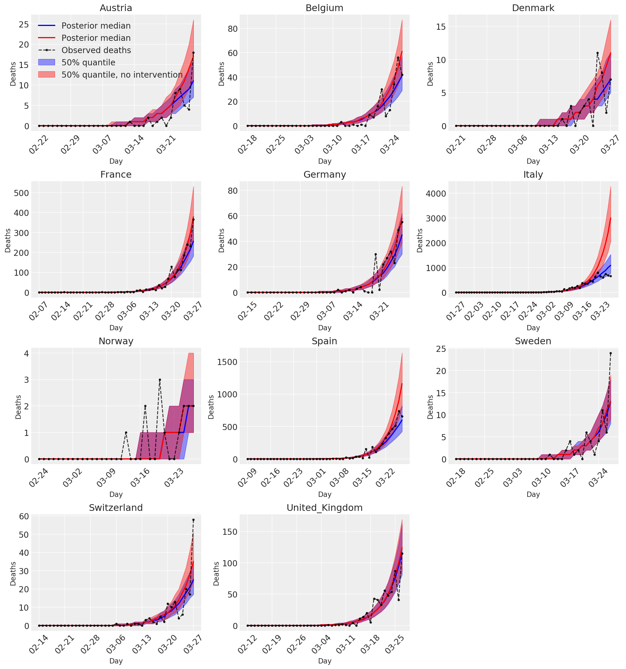
4.3 采取和不采取干预措施情况下的每日预测/预报的死亡人数
plot_quantile = True
forecast_days = 0

fig, ax = plt.subplots(4, 3, figsize=(15, 16))
ax = ax.flatten()
fig.delaxes(ax[-1])
for country_index, country in enumerate(COUNTRIES):
  num_days = (pd.to_datetime('2020-03-28') - first_days[country]).days + forecast_days
  dates = [(first_days[country] + i*pd.to_timedelta(1, 'days')).strftime('%m-%d') for i in range(num_days)]
  plot_dates = [dates[i] for i in range(0, num_days, 7)]

  ax[country_index].set_title(country)

  quantile_vals = [.025, .25, .5, .75, .975]
  samples = predicted_deaths[:, :, country_index].numpy()
  quantiles = []

  psi_m = psi_hat[np.newaxis, ..., np.newaxis]
  probs = tf.clip_by_value(expected_deaths / (expected_deaths + psi_m), 1e-9, 1.)
  predicted_deaths_dist = tfd.NegativeBinomial(
    total_count=psi_m, probs=probs)

  posterior_quantile = np.percentile(samples, [2.5, 25, 50, 75, 97.5], axis=-1)
  ax[country_index].plot(
      dates, posterior_quantile[2, :num_days],
      color='b', label='Posterior median', lw=2)
  if plot_quantile:
    ax[country_index].fill_between(
        dates, posterior_quantile[1, :num_days], posterior_quantile[3, :num_days],
        color='b', label='50% quantile', alpha=.4)

  samples_counterfact = no_intervention_predicted_deaths[:, :, country_index]
  posterior_quantile = np.percentile(samples_counterfact, [2.5, 25, 50, 75, 97.5], axis=-1)
  ax[country_index].plot(
      dates, posterior_quantile[2, :num_days],
      color='r', label='Posterior median', lw=2)
  if plot_quantile:
    ax[country_index].fill_between(
        dates, posterior_quantile[1, :num_days], posterior_quantile[3, :num_days],
        color='r', label='50% quantile, no intervention', alpha=.4)

  observed = deaths[country_index, :]
  observed[observed == -1] = np.nan
  ax[country_index].plot(
      dates, observed[:num_days],
      '--o', color='k', markersize=3,
      label='Observed deaths', alpha=.8)
  ax[country_index].set_xticks(plot_dates)
  ax[country_index].xaxis.set_tick_params(rotation=45)
  ax[country_index].set_title(country)
  ax[country_index].set_xlabel('Day', fontsize='large')
  ax[country_index].set_ylabel('Deaths', fontsize='large')
  ax[0].legend(loc='upper left')
plt.tight_layout(pad=1.0);