
ベイジアンモデルの選択
 GitHubでソースを表示 GitHubでソースを表示 |
インポート
import numpy as np
import tensorflow.compat.v2 as tf
tf.enable_v2_behavior()
import tensorflow_probability as tfp
from tensorflow_probability import distributions as tfd

from matplotlib import pylab as plt
%matplotlib inline
import scipy.stats
タスク: 複数の変化点を使用した変化点検出
変化点検出タスクについて考えてみます。イベントは、時間の経過とともに変動するレートで発生し、データを生成するシステムまたはプロセスの (監視されていない) 状態の突然の変化によって引き起こされます。
たとえば、次のような一連のカウントを観察する場合があります。
true_rates = [40, 3, 20, 50]
true_durations = [10, 20, 5, 35]

observed_counts = tf.concat(
    [tfd.Poisson(rate).sample(num_steps)
     for (rate, num_steps) in zip(true_rates, true_durations)], axis=0)

plt.plot(observed_counts)
[<matplotlib.lines.Line2D at 0x7f7589bdae10>]
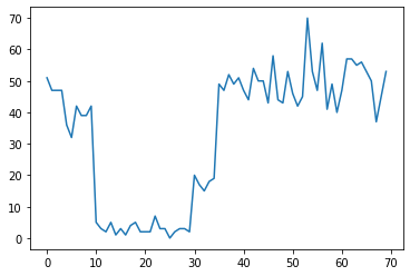
これらは、データセンターの障害の数、Web ページへの訪問者の数、ネットワークリンク上のパケットの数などを表す可能性があります。
データを見ただけでは、異なるシステム体制がいくつあるのかが明確ではないことに注意してください。3 つの変化点がそれぞれどこで発生するかわかりますか?
既知の状態数
まず、観測されていない状態の数が事前にわかっている (おそらく非現実的な) ケースを検討します。ここでは、4 つの潜在的な状態があることがわかっていると仮定します。
この問題を不均一ポアソン過程としてモデル化します。各時点で、発生するイベントの数はポアソン分布であり、イベントのレートは観測されていないシステム状態 \(z_t\) によって決定されます。
\[x_t \sim \text{Poisson}(\lambda_{z_t})\]
潜在状態は離散的 (\(z_t \in {1, 2, 3, 4}\)) です。したがって \(\lambda = [\lambda_1, \lambda_2, \lambda_3, \lambda_4]\) は、それぞれのポアソン比を含む単純なベクトルです。経時的な状態の変動をモデル化するために、単純な遷移モデル \(p(z_t | z_{t-1})\) を定義します。各ステップで、ある確率 \(p\) で前の状態にとどまるとしましょう。そして確率 \(1-p\) で、ランダムに均一に異なる状態に遷移します。初期状態もランダムに均一に選択されるため、次のようになります。
\[ \begin{align*} z_1 &\sim \text{Categorical}\left(\left{\frac{1}{4}, \frac{1}{4}, \frac{1}{4}, \frac{1}{4}\right}\right)\ z_t | z_{t-1} &\sim \text{Categorical}\left(\left{\begin{array}{cc}p & \text{if } z_t = z_{t-1} \ \frac{1-p}{4-1} & \text{otherwise}\end{array}\right}\right) \end{align*}\]
これらの仮定は、ポアソン放出を伴う隠れマルコフモデルに対応します。tfd.HiddenMarkovModel を使用して TFP でそれらをエンコードできます。最初に、初期状態の前に遷移行列と均一を定義します。
num_states = 4
initial_state_logits = tf.zeros([num_states]) # uniform distribution

daily_change_prob = 0.05
transition_probs = tf.fill([num_states, num_states],
                           daily_change_prob / (num_states - 1))
transition_probs = tf.linalg.set_diag(transition_probs,
                                      tf.fill([num_states],
                                              1 - daily_change_prob))

print("Initial state logits:\n{}".format(initial_state_logits))
print("Transition matrix:\n{}".format(transition_probs))
Initial state logits:
[0. 0. 0. 0.]
Transition matrix:
[[0.95       0.01666667 0.01666667 0.01666667]
 [0.01666667 0.95       0.01666667 0.01666667]
 [0.01666667 0.01666667 0.95       0.01666667]
 [0.01666667 0.01666667 0.01666667 0.95      ]]
次に、トレーニング可能な変数を使用して各システム状態に関連付けられたレートを表す tfd.HiddenMarkovModel 分布を作成します。レートが正の値になるように、対数空間でレートをパラメータ化します。
# Define variable to represent the unknown log rates.
trainable_log_rates = tf.Variable(
  tf.math.log(tf.reduce_mean(observed_counts)) +
  tf.random.stateless_normal([num_states], seed=(42, 42)),
  name='log_rates')

hmm = tfd.HiddenMarkovModel(
  initial_distribution=tfd.Categorical(
      logits=initial_state_logits),
  transition_distribution=tfd.Categorical(probs=transition_probs),
  observation_distribution=tfd.Poisson(log_rate=trainable_log_rates),
  num_steps=len(observed_counts))
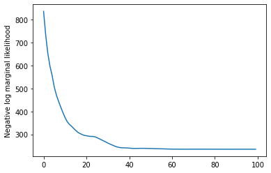
最後に、モデルの総対数密度を定義します。これには、レートの前の情報量の少ない LogNormal が含まれます。そして、オプティマイザを実行して、観測された計数データに適合する最大事後確率 (MAP) を計算します。
rate_prior = tfd.LogNormal(5, 5)

def log_prob():
 return (tf.reduce_sum(rate_prior.log_prob(tf.math.exp(trainable_log_rates))) +
         hmm.log_prob(observed_counts))

losses = tfp.math.minimize(
    lambda: -log_prob(),
    optimizer=tf.optimizers.Adam(learning_rate=0.1),
    num_steps=100)
plt.plot(losses)
plt.ylabel('Negative log marginal likelihood')
Text(0, 0.5, 'Negative log marginal likelihood')
rates = tf.exp(trainable_log_rates)
print("Inferred rates: {}".format(rates))
print("True rates: {}".format(true_rates))
Inferred rates: [ 2.8302798 49.58499   41.928307  17.35112  ]
True rates: [40, 3, 20, 50]
上手くいきました。このモデルの潜在状態は順列までしか識別できないため、回復したレートの順序は異なり、ノイズが少しありますが、一般的にはかなりよく一致しているます。
状態の軌道を回復する
モデルを適合させたので、各タイムステップで存在するとモデルが考えているシステムの状態を再構築します。
これは事後推論タスクです。観測されたカウント \(x_{1:T}\) とモデルパラメータ (レート) \(\lambda\) が与えられた場合、事後分布 \(p(z_{1:T} | x_{1:T}, \lambda)\) に従って離散潜在変数のシーケンスを推論します。隠れマルコフモデルでは、標準のメッセージパッシングアルゴリズムを使用して、この分布の周辺分布やその他のプロパティを効率的に計算できます。特に、posterior_marginals メソッドは、(前方後方アルゴリズムを使用して) 各タイムステップ \(t\) での離散潜在状態 \(Z_t\) の周辺確率分布 \(p(Z_t = z_t | x_{1:T})\) を効率的に計算します。
# Runs forward-backward algorithm to compute marginal posteriors.
posterior_dists = hmm.posterior_marginals(observed_counts)
posterior_probs = posterior_dists.probs_parameter().numpy()
事後確率をプロットして、モデルのデータの「説明」を復元します。各状態がアクティブになっているのはどの時点でしょうか。
def plot_state_posterior(ax, state_posterior_probs, title):
  ln1 = ax.plot(state_posterior_probs, c='blue', lw=3, label='p(state | counts)')
  ax.set_ylim(0., 1.1)
  ax.set_ylabel('posterior probability')
  ax2 = ax.twinx()
  ln2 = ax2.plot(observed_counts, c='black', alpha=0.3, label='observed counts')
  ax2.set_title(title)
  ax2.set_xlabel("time")
  lns = ln1+ln2
  labs = [l.get_label() for l in lns]
  ax.legend(lns, labs, loc=4)
  ax.grid(True, color='white')
  ax2.grid(False)

fig = plt.figure(figsize=(10, 10))
plot_state_posterior(fig.add_subplot(2, 2, 1),
                     posterior_probs[:, 0],
                     title="state 0 (rate {:.2f})".format(rates[0]))
plot_state_posterior(fig.add_subplot(2, 2, 2),
                     posterior_probs[:, 1],
                     title="state 1 (rate {:.2f})".format(rates[1]))
plot_state_posterior(fig.add_subplot(2, 2, 3),
                     posterior_probs[:, 2],
                     title="state 2 (rate {:.2f})".format(rates[2]))
plot_state_posterior(fig.add_subplot(2, 2, 4),
                     posterior_probs[:, 3],
                     title="state 3 (rate {:.2f})".format(rates[3]))
plt.tight_layout()
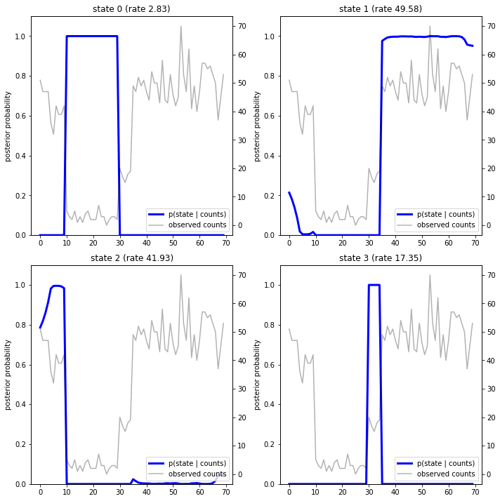
この (単純な) ケースでは、モデルは通常信頼度が高いことがわかります。ほとんどのタイムステップで、基本的にすべての確率質量が 4 つの状態の 1 つに割り当てられます。幸いなことに、説明は合理的に見えます。
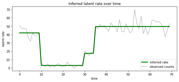
また、各タイムステップで最も可能性の高い潜在状態に関連付けられたレートの観点からこの事後確率を視覚化し、事後確率を 1 つの説明にまとめることもできます。
most_probable_states = hmm.posterior_mode(observed_counts)
most_probable_rates = tf.gather(rates, most_probable_states)
fig = plt.figure(figsize=(10, 4))
ax = fig.add_subplot(1, 1, 1)
ax.plot(most_probable_rates, c='green', lw=3, label='inferred rate')
ax.plot(observed_counts, c='black', alpha=0.3, label='observed counts')
ax.set_ylabel("latent rate")
ax.set_xlabel("time")
ax.set_title("Inferred latent rate over time")
ax.legend(loc=4)
<matplotlib.legend.Legend at 0x7f75849e70f0>
状態の数が不明
実際の問題では、モデル化しているシステムの「真の」状態の数がわからない場合があります。これは常に問題になるわけではありません。不明な状態の ID を特に気にしない場合は、モデルに必要な数よりも多くの状態でモデルを実行し、実際の状態の多数の重複コピーを学習することができます。しかし、潜在状態の「真の」数を推測することに注意を払っていると仮定しましょう。
これは、ベイジアンモデル選択の場合と見なすことができます。候補モデルのセットがあり、それぞれに潜在状態の数が異なり、観測されたデータを生成した可能性が最も高いモデルを選択します。これを行うために、各モデルの下でデータの周辺尤度を計算します (モデル自体に事前分布を追加することもできますが、この分析では必要ありません。ベイジアンオッカムの剃刀はより単純なモデルへの選好をエンコードするのに十分です)。
残念ながら、離散状態 \(z_{1:T}\) とレートパラメータ (のベクトル) \( \ lambda \)、 \(\lambda\), \(p(x_{1:T}) = \int p(x_{1:T}, z_{1:T}, \lambda) dz d\lambda,\) は、このモデルでは使用できません。便宜上、いわゆる「経験的ベイズ」または「タイプ II 最尤」推定を使用して概算します。関連する (不明な) レートパラメータ \(\lambda\) を完全に統合する代わりに各システム状態について、それらの値を最適化します。
\[\tilde{p}(x_{1:T}) = \max_\lambda \int p(x_{1:T}, z_{1:T}, \lambda) dz\]
この近似は過適合する可能性があります。つまり、真の周辺尤度よりも複雑なモデルを優先します。より忠実な近似を検討できます。たとえば、変分下限を最適化するか、アニーリング重要度サンプリングなどのモンテカルロ推定量を使用します。これらはこのノートブックでは取り上げません。(ベイズモデルの選択と近似の詳細については機械学習:確率論的視点の第 7 章を参照してください。)
原則として、num_states の値を変えて上記の最適化を何度も再実行するだけで、このモデルの比較を行うことができますが、それは大変な作業になります。ここでは、ベクトル化に TFP の batch_shape メカニズムを使用して、複数のモデルを並行して検討する方法を示します。
遷移行列と事前の初期状態: 単一のモデル記述を作成するのではなく、遷移行列と以前のロジットの{nbsp}バッチを、max_num_states までの候補モデルごとに 1 つずつ作成します。バッチ処理を簡単にするには、すべての計算が同じ「形状」であることを確認する必要があります。これは、適合する最大のモデルの寸法に対応している必要があります。より小さなモデルを処理するために、状態空間の最上位の次元にそれらの説明を「埋め込み」、残りの次元を使用されることのないダミー状態として効果的に扱うことができます。
max_num_states = 10

def build_latent_state(num_states, max_num_states, daily_change_prob=0.05):

  # Give probability exp(-100) ~= 0 to states outside of the current model.
  active_states_mask = tf.concat([tf.ones([num_states]),
                                  tf.zeros([max_num_states - num_states])],
                                 axis=0)
  initial_state_logits = -100. * (1 - active_states_mask)

  # Build a transition matrix that transitions only within the current
  # `num_states` states.
  transition_probs = tf.fill([num_states, num_states],
                             0. if num_states == 1
                             else daily_change_prob / (num_states - 1))
  padded_transition_probs = tf.eye(max_num_states) + tf.pad(
      tf.linalg.set_diag(transition_probs,
                         tf.fill([num_states], - daily_change_prob)),
      paddings=[(0, max_num_states - num_states),
                (0, max_num_states - num_states)])

  return initial_state_logits, padded_transition_probs

# For each candidate model, build the initial state prior and transition matrix.
batch_initial_state_logits = []
batch_transition_probs = []
for num_states in range(1, max_num_states+1):
  initial_state_logits, transition_probs = build_latent_state(
      num_states=num_states,
      max_num_states=max_num_states)
  batch_initial_state_logits.append(initial_state_logits)
  batch_transition_probs.append(transition_probs)

batch_initial_state_logits = tf.stack(batch_initial_state_logits)
batch_transition_probs = tf.stack(batch_transition_probs)
print("Shape of initial_state_logits: {}".format(batch_initial_state_logits.shape))
print("Shape of transition probs: {}".format(batch_transition_probs.shape))
print("Example initial state logits for num_states==3:\n{}".format(batch_initial_state_logits[2, :]))
print("Example transition_probs for num_states==3:\n{}".format(batch_transition_probs[2, :, :]))
Shape of initial_state_logits: (10, 10)
Shape of transition probs: (10, 10, 10)
Example initial state logits for num_states==3:
[  -0.   -0.   -0. -100. -100. -100. -100. -100. -100. -100.]
Example transition_probs for num_states==3:
[[0.95  0.025 0.025 0.    0.    0.    0.    0.    0.    0.   ]
 [0.025 0.95  0.025 0.    0.    0.    0.    0.    0.    0.   ]
 [0.025 0.025 0.95  0.    0.    0.    0.    0.    0.    0.   ]
 [0.    0.    0.    1.    0.    0.    0.    0.    0.    0.   ]
 [0.    0.    0.    0.    1.    0.    0.    0.    0.    0.   ]
 [0.    0.    0.    0.    0.    1.    0.    0.    0.    0.   ]
 [0.    0.    0.    0.    0.    0.    1.    0.    0.    0.   ]
 [0.    0.    0.    0.    0.    0.    0.    1.    0.    0.   ]
 [0.    0.    0.    0.    0.    0.    0.    0.    1.    0.   ]
 [0.    0.    0.    0.    0.    0.    0.    0.    0.    1.   ]]
上記と同様に進みます。ここでは trainable_rates で追加のバッチ次元を使用して、検討中の各モデルのレートを個別に適合させます。
trainable_log_rates = tf.Variable(
    tf.fill([batch_initial_state_logits.shape[0], max_num_states],
            tf.math.log(tf.reduce_mean(observed_counts))) +
     tf.random.stateless_normal([1, max_num_states], seed=(42, 42)),
     name='log_rates')

hmm = tfd.HiddenMarkovModel(
  initial_distribution=tfd.Categorical(
      logits=batch_initial_state_logits),
  transition_distribution=tfd.Categorical(probs=batch_transition_probs),
  observation_distribution=tfd.Poisson(log_rate=trainable_log_rates),
  num_steps=len(observed_counts))
print("Defined HMM with batch shape: {}".format(hmm.batch_shape))
Defined HMM with batch shape: (10,)
対数確率の合計値を計算する際には、各モデル成分で実際に使用されるレートの事前確率のみを合計するように注意します。
rate_prior = tfd.LogNormal(5, 5)

def log_prob():
  prior_lps = rate_prior.log_prob(tf.math.exp(trainable_log_rates))
  prior_lp = tf.stack(
      [tf.reduce_sum(prior_lps[i, :i+1]) for i in range(max_num_states)])
  return prior_lp + hmm.log_prob(observed_counts)
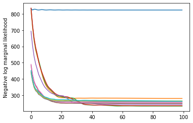
次に、構築したバッチ目標を最適化し、すべての候補モデルを同時に適合させます。
losses = tfp.math.minimize(
    lambda: -log_prob(),
    optimizer=tf.optimizers.Adam(0.1),
    num_steps=100)
plt.plot(losses)
plt.ylabel('Negative log marginal likelihood')
Text(0, 0.5, 'Negative log marginal likelihood')
num_states = np.arange(1, max_num_states+1)
plt.plot(num_states, -losses[-1])
plt.ylim([-400, -200])
plt.ylabel("marginal likelihood $\\tilde{p}(x)$")
plt.xlabel("number of latent states")
plt.title("Model selection on latent states")
Text(0.5, 1.0, 'Model selection on latent states')
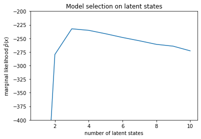
尤度を調べると、(おおよその) 周辺尤度が 3 つの状態モデルを好むことがわかります。これは妥当です。「真の」モデルには 4 つの状態がありましたが、データを見るだけでは、3 つの状態の説明を除外することは困難です。
また、各候補モデルに適合するレートを抽出することもできます。
rates = tf.exp(trainable_log_rates)
for i, learned_model_rates in enumerate(rates):
  print("rates for {}-state model: {}".format(i+1, learned_model_rates[:i+1]))
rates for 1-state model: [32.968506]
rates for 2-state model: [ 5.789209 47.948917]
rates for 3-state model: [ 2.841977 48.057507 17.958897]
rates for 4-state model: [ 2.8302798 49.585037  41.928406  17.351114 ]
rates for 5-state model: [17.399694  77.83679   41.975216  49.62771    2.8256145]
rates for 6-state model: [41.63677   77.20768   49.570934  49.557076  17.630419   2.8713436]
rates for 7-state model: [41.711704  76.405945  49.581184  49.561283  17.451889   2.8722699
 17.43608  ]
rates for 8-state model: [41.771793 75.41323  49.568714 49.591846 17.2523   17.247969 17.231388
  2.830598]
rates for 9-state model: [41.83378   74.50916   49.619488  49.622494   2.8369408 17.254414
 17.21532    2.5904858 17.252514 ]
rates for 10-state model: [4.1886074e+01 7.3912338e+01 4.1940136e+01 4.9652588e+01 2.8485537e+00
 1.7433832e+01 6.7564294e-02 1.9590002e+00 1.7430998e+01 7.8838937e-02]
そして、各モデルがデータに対して提供する説明をプロットします。
most_probable_states = hmm.posterior_mode(observed_counts)
fig = plt.figure(figsize=(14, 12))
for i, learned_model_rates in enumerate(rates):
  ax = fig.add_subplot(4, 3, i+1)
  ax.plot(tf.gather(learned_model_rates, most_probable_states[i]), c='green', lw=3, label='inferred rate')
  ax.plot(observed_counts, c='black', alpha=0.3, label='observed counts')
  ax.set_ylabel("latent rate")
  ax.set_xlabel("time")
  ax.set_title("{}-state model".format(i+1))
  ax.legend(loc=4)
plt.tight_layout()
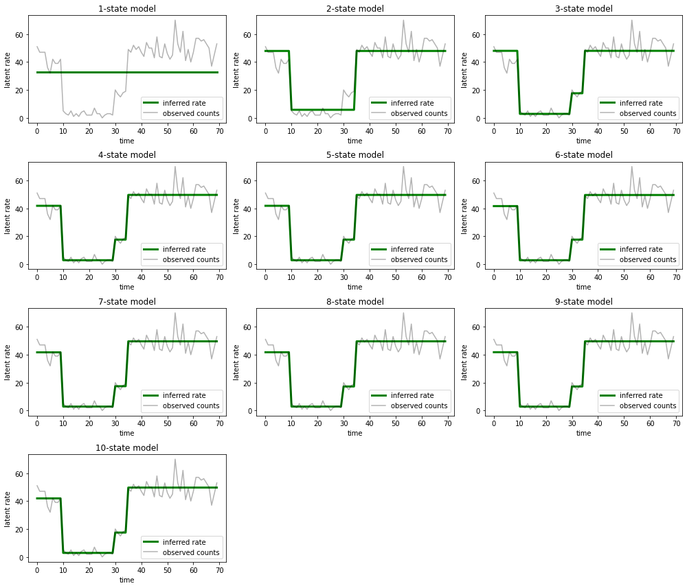
1 つの状態、2 つの状態、および (より微妙ながら) 3 つの状態のモデルによる説明が不適切であることを簡単に理解できます。興味深いことに、4 つの状態を超えるすべてのモデルは、本質的に同じ説明を提供します。これは、「データ」が比較的クリーンであり、代替の説明の余地がほとんどないためと考えられます。より乱雑な実世界のデータでは、大きなモデルがデータへの適合性を徐々に向上させることが期待されますが、モデルの複雑さの方が適合性の向上よりも重要視されるというトレードオフがあります。
拡張機能
このノートブックのモデルは、さまざまな方法で簡単に拡張できます。例えば、
- 潜在状態が異なる確率を持つことを許可する (一部の状態は一般的であるかまれである可能性があります)。
- 潜在的な状態間の不均一な遷移を許可する(たとえば、マシンのクラッシュの後に通常はシステムの再起動が続き、通常は良好なパフォーマンスの期間が続くことを学習するなど)
- 他のエミッションモデル (たとえば、
NegativeBinomialは、カウントデータのさまざまな分散、または実数値データのNormalなどの連続分布をモデル化します)。