| | |  צפה במקור ב-GitHub צפה במקור ב-GitHub | |
מחברת זו מדגים את השימוש בכלי הסקה משוערים של TFP כדי לשלב מודל תצפית (לא גאוסי) בעת התאמה וחיזוי של מודלים של סדרות זמן מבניות (STS). בדוגמה זו, נשתמש במודל תצפית של Poisson כדי לעבוד עם נתוני ספירה בדידים.
import time
import matplotlib.pyplot as plt
import numpy as np

import tensorflow.compat.v2 as tf
import tensorflow_probability as tfp

from tensorflow_probability import bijectors as tfb
from tensorflow_probability import distributions as tfd

tf.enable_v2_behavior()
נתונים סינתטיים
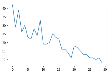
ראשית, ניצור כמה נתוני ספירה סינתטיים:
num_timesteps = 30
observed_counts = np.round(3 + np.random.lognormal(np.log(np.linspace(
    num_timesteps, 5, num=num_timesteps)), 0.20, size=num_timesteps))
observed_counts = observed_counts.astype(np.float32)
plt.plot(observed_counts)
[<matplotlib.lines.Line2D at 0x7f940ae958d0>]
דֶגֶם
נציין מודל פשוט עם מגמה לינארית מהלכת באופן אקראי:
def build_model(approximate_unconstrained_rates):
  trend = tfp.sts.LocalLinearTrend(
      observed_time_series=approximate_unconstrained_rates)
  return tfp.sts.Sum([trend],
                     observed_time_series=approximate_unconstrained_rates)
במקום לפעול על סדרת הזמן הנצפית, מודל זה יפעל על סדרת הפרמטרים של קצב הפואסון השולטים בתצפיות.
מכיוון ששיעורי Poisson חייבים להיות חיוביים, נשתמש בביקטור כדי להפוך את מודל STS בעל הערך האמיתי להתפלגות על פני ערכים חיוביים. Softplus טרנספורמציה \(y = \log(1 + \exp(x))\) הוא בחירה טבעית, שכן הוא כמעט ליניארי עבור ערכים חיוביים, אך ברירות אחרות כגון Exp (אשר הופך ההילוך המקרי הנורמלי עברה להליכת lognormal אקראית) הם גם אפשריות.
positive_bijector = tfb.Softplus()  # Or tfb.Exp()

# Approximate the unconstrained Poisson rate just to set heuristic priors.
# We could avoid this by passing explicit priors on all model params.
approximate_unconstrained_rates = positive_bijector.inverse(
    tf.convert_to_tensor(observed_counts) + 0.01)
sts_model = build_model(approximate_unconstrained_rates)
כדי להשתמש בהסקה משוערת עבור מודל תצפית לא גאוסי, נקודד את מודל STS כ-TFP JointDistribution. המשתנים האקראיים בהתפלגות משותפת זו הם הפרמטרים של מודל STS, סדרת הזמן של שיעורי פויסון סמויים והספירות הנצפות.
def sts_with_poisson_likelihood_model():
  # Encode the parameters of the STS model as random variables.
  param_vals = []
  for param in sts_model.parameters:
    param_val = yield param.prior
    param_vals.append(param_val)

  # Use the STS model to encode the log- (or inverse-softplus)
  # rate of a Poisson.
  unconstrained_rate = yield sts_model.make_state_space_model(
      num_timesteps, param_vals)
  rate = positive_bijector.forward(unconstrained_rate[..., 0])
  observed_counts = yield tfd.Poisson(rate, name='observed_counts')

model = tfd.JointDistributionCoroutineAutoBatched(sts_with_poisson_likelihood_model)
הכנה להסקת מסקנות
אנו רוצים להסיק את הכמויות שלא נצפו במודל, בהינתן הספירות שנצפו. ראשית, אנו מתנים את צפיפות היומן המפרק בספירות שנצפו.
pinned_model = model.experimental_pin(observed_counts=observed_counts)
נזדקק גם לביקטור מגביל כדי להבטיח שהמסק מכבד את האילוצים על הפרמטרים של מודל STS (לדוגמה, קנה מידה חייב להיות חיובי).
constraining_bijector = pinned_model.experimental_default_event_space_bijector()
הסקה עם HMC
נשתמש ב-HMC (באופן ספציפי, NUTS) כדי לדגום מהמפרק האחורי על פני פרמטרים של מודל וקצבים סמויים.
זה יהיה איטי משמעותית מהתאמת דגם STS סטנדרטי עם HMC, שכן בנוסף לפרמטרים (היחסית הקטן של) של הדגם עלינו להסיק את כל סדרת שיעורי ה-Poisson. אז נרוץ למספר קטן יחסית של צעדים; עבור יישומים שבהם איכות ההסקה היא קריטית, עשוי להיות הגיוני להגדיל את הערכים הללו או להפעיל רשתות מרובות.
תצורת דגימה
# Allow external control of sampling to reduce test runtimes.
num_results = 500 # @param { isTemplate: true}
num_results = int(num_results)

num_burnin_steps = 100 # @param { isTemplate: true}
num_burnin_steps = int(num_burnin_steps)
ראשית נגדיר סמפלר, ולאחר מכן להשתמש sample_chain לרוץ כי הקרנל דגימה כדי דגימות תוצרת.
sampler = tfp.mcmc.TransformedTransitionKernel(
    tfp.mcmc.NoUTurnSampler(
        target_log_prob_fn=pinned_model.unnormalized_log_prob,
        step_size=0.1),
    bijector=constraining_bijector)

adaptive_sampler = tfp.mcmc.DualAveragingStepSizeAdaptation(
    inner_kernel=sampler,
    num_adaptation_steps=int(0.8 * num_burnin_steps),
    target_accept_prob=0.75)

initial_state = constraining_bijector.forward(
    type(pinned_model.event_shape)(
        *(tf.random.normal(part_shape)
          for part_shape in constraining_bijector.inverse_event_shape(
              pinned_model.event_shape))))
# Speed up sampling by tracing with `tf.function`.
@tf.function(autograph=False, jit_compile=True)
def do_sampling():
  return tfp.mcmc.sample_chain(
      kernel=adaptive_sampler,
      current_state=initial_state,
      num_results=num_results,
      num_burnin_steps=num_burnin_steps,
      trace_fn=None)

t0 = time.time()
samples = do_sampling()
t1 = time.time()
print("Inference ran in {:.2f}s.".format(t1-t0))
Inference ran in 24.83s.
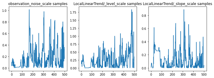
אנחנו יכולים לבדוק את ההסקה על ידי שפיות על ידי בחינת עקבות הפרמטרים. במקרה זה נראה שהם בחנו מספר הסברים לנתונים, וזה טוב, אם כי דגימות נוספות יעזרו לשפוט עד כמה השרשרת מתערבבת.
f = plt.figure(figsize=(12, 4))
for i, param in enumerate(sts_model.parameters):
  ax = f.add_subplot(1, len(sts_model.parameters), i + 1)
  ax.plot(samples[i])
  ax.set_title("{} samples".format(param.name))
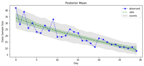
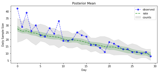
עכשיו לתמורה: בוא נראה את שיעורי הפואסון האחוריים! אנו גם נשרטט את המרווח הניבוי של 80% על פני ספירות שנצפו, ונוכל לבדוק שנראה שמרווח זה מכיל כ-80% מהספירות שצפינו בפועל.
param_samples = samples[:-1]
unconstrained_rate_samples = samples[-1][..., 0]
rate_samples = positive_bijector.forward(unconstrained_rate_samples)

plt.figure(figsize=(10, 4))
mean_lower, mean_upper = np.percentile(rate_samples, [10, 90], axis=0)
pred_lower, pred_upper = np.percentile(np.random.poisson(rate_samples),
                                       [10, 90], axis=0)

_ = plt.plot(observed_counts, color="blue", ls='--', marker='o', label='observed', alpha=0.7)
_ = plt.plot(np.mean(rate_samples, axis=0), label='rate', color="green", ls='dashed', lw=2, alpha=0.7)
_ = plt.fill_between(np.arange(0, 30), mean_lower, mean_upper, color='green', alpha=0.2)
_ = plt.fill_between(np.arange(0, 30), pred_lower, pred_upper, color='grey', label='counts', alpha=0.2)
plt.xlabel("Day")
plt.ylabel("Daily Sample Size")
plt.title("Posterior Mean")
plt.legend()
<matplotlib.legend.Legend at 0x7f93ffd35550>
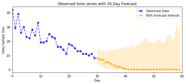
חיזוי
כדי לחזות את הספירות הנצפות, נשתמש בכלי ה-STS הסטנדרטיים כדי לבנות התפלגות תחזית על הקצבים הסמויים (במרחב בלתי מוגבל, שוב מכיוון ש-STS נועד למודל נתונים בעלי ערך אמיתי), ולאחר מכן נעביר את התחזיות הנדגמות דרך תצפית Poisson דֶגֶם:
def sample_forecasted_counts(sts_model, posterior_latent_rates,
                             posterior_params, num_steps_forecast,
                             num_sampled_forecasts):

  # Forecast the future latent unconstrained rates, given the inferred latent
  # unconstrained rates and parameters.
  unconstrained_rates_forecast_dist = tfp.sts.forecast(sts_model,
    observed_time_series=unconstrained_rate_samples,
    parameter_samples=posterior_params,
    num_steps_forecast=num_steps_forecast)

  # Transform the forecast to positive-valued Poisson rates.
  rates_forecast_dist = tfd.TransformedDistribution(
      unconstrained_rates_forecast_dist,
      positive_bijector)

  # Sample from the forecast model following the chain rule:
  # P(counts) = P(counts | latent_rates)P(latent_rates)
  sampled_latent_rates = rates_forecast_dist.sample(num_sampled_forecasts)
  sampled_forecast_counts = tfd.Poisson(rate=sampled_latent_rates).sample()

  return sampled_forecast_counts, sampled_latent_rates

forecast_samples, rate_samples = sample_forecasted_counts(
   sts_model,
   posterior_latent_rates=unconstrained_rate_samples,
   posterior_params=param_samples,
   # Days to forecast:
   num_steps_forecast=30,
   num_sampled_forecasts=100)
forecast_samples = np.squeeze(forecast_samples)
def plot_forecast_helper(data, forecast_samples, CI=90):
"""Plot the observed time series alongside the forecast."""
plt.figure(figsize=(10, 4))
forecast_median = np.median(forecast_samples, axis=0)
num_steps = len(data)
num_steps_forecast = forecast_median.shape[-1]
plt.plot(np.arange(num_steps), data, lw=2, color='blue', linestyle='--', marker='o',
label='Observed Data', alpha=0.7)
forecast_steps = np.arange(num_steps, num_steps+num_steps_forecast)
CI_interval = [(100 - CI)/2, 100 - (100 - CI)/2]
lower, upper = np.percentile(forecast_samples, CI_interval, axis=0)
plt.plot(forecast_steps, forecast_median, lw=2, ls='--', marker='o', color='orange',
label=str(CI) + '% Forecast Interval', alpha=0.7)
plt.fill_between(forecast_steps,
lower,
upper, color='orange', alpha=0.2)
plt.xlim([0, num_steps+num_steps_forecast])
ymin, ymax = min(np.min(forecast_samples), np.min(data)), max(np.max(forecast_samples), np.max(data))
yrange = ymax-ymin
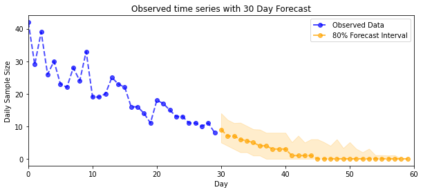
plt.title("{}".format('Observed time series with ' + str(num_steps_forecast) + ' Day Forecast'))
plt.xlabel('Day')
plt.ylabel('Daily Sample Size')
plt.legend()
plot_forecast_helper(observed_counts, forecast_samples, CI=80)
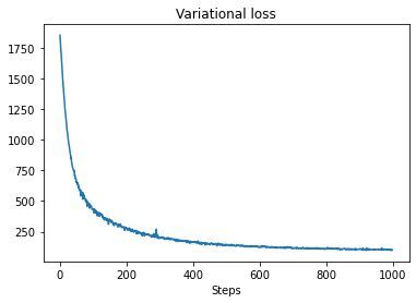
מסקנות VI
היקש וריאציה יכול להיות בעייתי כאשר הסיק סדרה במשרה מלאה, כמו ספירת המשוער שלנו (להבדיל רק לפרמטרים של סדרת זמן, כמו מודלים STS סטנדרטי). ההנחה הסטנדרטית שלמשתנים יש אחוריים בלתי תלויים היא שגויה למדי, שכן כל צעד זמן נמצא בקורלציה עם שכנותיו, מה שעלול להוביל לחוסר הערכת אי ודאות. מסיבה זו, HMC עשויה להיות בחירה טובה יותר להסקה משוערת על פני סדרות מלאות. עם זאת, VI יכול להיות די מהיר יותר, ועשוי להיות שימושי עבור יצירת אב טיפוס של מודלים או במקרים שבהם ניתן להוכיח אמפירית שהביצועים שלו הם 'טובים מספיק'.
כדי להתאים את המודל שלנו ל-VI, אנו פשוט בונים ומייעלים פוסטריור פוסטריורי:
surrogate_posterior = tfp.experimental.vi.build_factored_surrogate_posterior(
    event_shape=pinned_model.event_shape,
    bijector=constraining_bijector)
# Allow external control of optimization to reduce test runtimes.
num_variational_steps = 1000 # @param { isTemplate: true}
num_variational_steps = int(num_variational_steps)

t0 = time.time()
losses = tfp.vi.fit_surrogate_posterior(pinned_model.unnormalized_log_prob,
                                        surrogate_posterior,
                                        optimizer=tf.optimizers.Adam(0.1),
                                        num_steps=num_variational_steps)
t1 = time.time()
print("Inference ran in {:.2f}s.".format(t1-t0))
Inference ran in 11.37s.
plt.plot(losses)
plt.title("Variational loss")
_ = plt.xlabel("Steps")
posterior_samples = surrogate_posterior.sample(50)
param_samples = posterior_samples[:-1]
unconstrained_rate_samples = posterior_samples[-1][..., 0]
rate_samples = positive_bijector.forward(unconstrained_rate_samples)

plt.figure(figsize=(10, 4))
mean_lower, mean_upper = np.percentile(rate_samples, [10, 90], axis=0)
pred_lower, pred_upper = np.percentile(
    np.random.poisson(rate_samples), [10, 90], axis=0)

_ = plt.plot(observed_counts, color='blue', ls='--', marker='o',
             label='observed', alpha=0.7)
_ = plt.plot(np.mean(rate_samples, axis=0), label='rate', color='green',
             ls='dashed', lw=2, alpha=0.7)
_ = plt.fill_between(
    np.arange(0, 30), mean_lower, mean_upper, color='green', alpha=0.2)
_ = plt.fill_between(np.arange(0, 30), pred_lower, pred_upper, color='grey',
    label='counts', alpha=0.2)
plt.xlabel('Day')
plt.ylabel('Daily Sample Size')
plt.title('Posterior Mean')
plt.legend()
<matplotlib.legend.Legend at 0x7f93ff4735c0>
forecast_samples, rate_samples = sample_forecasted_counts(
   sts_model,
   posterior_latent_rates=unconstrained_rate_samples,
   posterior_params=param_samples,
   # Days to forecast:
   num_steps_forecast=30,
   num_sampled_forecasts=100)
forecast_samples = np.squeeze(forecast_samples)
plot_forecast_helper(observed_counts, forecast_samples, CI=80)