GitHub でソースを表示 GitHub でソースを表示 |
このノートブックでは、構造時系列(STS)モデルで適合と予測を行う際に、(非ガウス型)観測モデルを取り込む上で TFP 禁じ推論ツールを使用する方法を説明します。この例では、ポワソン方観測モデルを使用して、離散カウントデータを操作します。
import time
import matplotlib.pyplot as plt
import numpy as np

import tensorflow.compat.v2 as tf
import tensorflow_probability as tfp

from tensorflow_probability import bijectors as tfb
from tensorflow_probability import distributions as tfd

tf.enable_v2_behavior()
合成データ
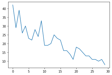
まず、合成カウントデータを生成します。
num_timesteps = 30
observed_counts = np.round(3 + np.random.lognormal(np.log(np.linspace(
    num_timesteps, 5, num=num_timesteps)), 0.20, size=num_timesteps))
observed_counts = observed_counts.astype(np.float32)
plt.plot(observed_counts)
[<matplotlib.lines.Line2D at 0x7f940ae958d0>]
モデル
ランダムウォーク線形トレンドを使用して、単純なモデルを指定します。
def build_model(approximate_unconstrained_rates):
  trend = tfp.sts.LocalLinearTrend(
      observed_time_series=approximate_unconstrained_rates)
  return tfp.sts.Sum([trend],
                     observed_time_series=approximate_unconstrained_rates)
このモデルは、観測された時系列で演算する代わりに、観測を管理するポワソン型レートパラメータの系列で演算します。
ポワソン型レートは正である必要があるため、バイジェクターを使用して、正値に渡って実際値の STS モデルを分布に変換します。Softplus 変換の \(y = \log(1 + \exp(x))\) は正の値がほぼ線形であるため、自然な選択と言えますが、ほかの Exp(通常のランダムウォークを対数正規ランダムウォークに変換します)といった選択肢でも可能です。
positive_bijector = tfb.Softplus()  # Or tfb.Exp()

# Approximate the unconstrained Poisson rate just to set heuristic priors.
# We could avoid this by passing explicit priors on all model params.
approximate_unconstrained_rates = positive_bijector.inverse(
    tf.convert_to_tensor(observed_counts) + 0.01)
sts_model = build_model(approximate_unconstrained_rates)
非ガウス型観測モデルに近似推論を使用するために、STS モデルを TFP JointDistribution としてエンコーディングします。この同時分布の確率変数は STS モデル、潜在ポワソン分布レートの時系列、および観測されたカウントのパラメータです。
def sts_with_poisson_likelihood_model():
  # Encode the parameters of the STS model as random variables.
  param_vals = []
  for param in sts_model.parameters:
    param_val = yield param.prior
    param_vals.append(param_val)

  # Use the STS model to encode the log- (or inverse-softplus)
  # rate of a Poisson.
  unconstrained_rate = yield sts_model.make_state_space_model(
      num_timesteps, param_vals)
  rate = positive_bijector.forward(unconstrained_rate[..., 0])
  observed_counts = yield tfd.Poisson(rate, name='observed_counts')

model = tfd.JointDistributionCoroutineAutoBatched(sts_with_poisson_likelihood_model)
推論の準備
指定された観測数で、モデル内の未観測の数量を推論します。まず、観測数に同時対数密度を条件づけます。
pinned_model = model.experimental_pin(observed_counts=observed_counts)
また、推論が STS モデルのパラメータへの制約(スケールが正であるなど)を考慮するように、制約付きのバイジェクターも必要です。
constraining_bijector = pinned_model.experimental_default_event_space_bijector()
HMC による推論
HMC(特に NUTS)を使用して、モデルパラメータと潜在レートでの同時事後分布からサンプリングします。
これは、HMC で標準 STS モデルを適合するよりもはるかに低速化します。モデルの(相対的に少ない数の)パラメータのほかに、ポワソン分布レートの全系列も推論しなくてはいけないためです。そのため、相対的に少ないステップ数に実行することにします。推論の質が重要となるアプリケーションについては、これらの値を増加するか複数のチェーンを実行するのが合理的です。
Sampler configuration
# Allow external control of sampling to reduce test runtimes.
num_results = 500 # @param { isTemplate: true}
num_results = int(num_results)

num_burnin_steps = 100 # @param { isTemplate: true}
num_burnin_steps = int(num_burnin_steps)
まず、サンプラーを指定し、sample_chain を使用してサンプルを生成するサンプリングカーネルを実行します。
sampler = tfp.mcmc.TransformedTransitionKernel(
    tfp.mcmc.NoUTurnSampler(
        target_log_prob_fn=pinned_model.unnormalized_log_prob,
        step_size=0.1),
    bijector=constraining_bijector)

adaptive_sampler = tfp.mcmc.DualAveragingStepSizeAdaptation(
    inner_kernel=sampler,
    num_adaptation_steps=int(0.8 * num_burnin_steps),
    target_accept_prob=0.75)

initial_state = constraining_bijector.forward(
    type(pinned_model.event_shape)(
        *(tf.random.normal(part_shape)
          for part_shape in constraining_bijector.inverse_event_shape(
              pinned_model.event_shape))))
# Speed up sampling by tracing with `tf.function`.
@tf.function(autograph=False, jit_compile=True)
def do_sampling():
  return tfp.mcmc.sample_chain(
      kernel=adaptive_sampler,
      current_state=initial_state,
      num_results=num_results,
      num_burnin_steps=num_burnin_steps,
      trace_fn=None)

t0 = time.time()
samples = do_sampling()
t1 = time.time()
print("Inference ran in {:.2f}s.".format(t1-t0))
Inference ran in 24.83s.
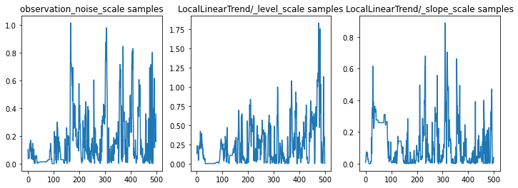
パラメータのトレースを調べて、推論のサニティチェックを行います。この場合、データに対し複数の説明が探られたようです。これは良いことではありますが、サンプルが多いほどチェーンの混合状態がどれだけうまく行っているかを判定しやすくなります。
f = plt.figure(figsize=(12, 4))
for i, param in enumerate(sts_model.parameters):
  ax = f.add_subplot(1, len(sts_model.parameters), i + 1)
  ax.plot(samples[i])
  ax.set_title("{} samples".format(param.name))
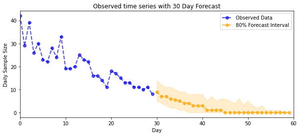
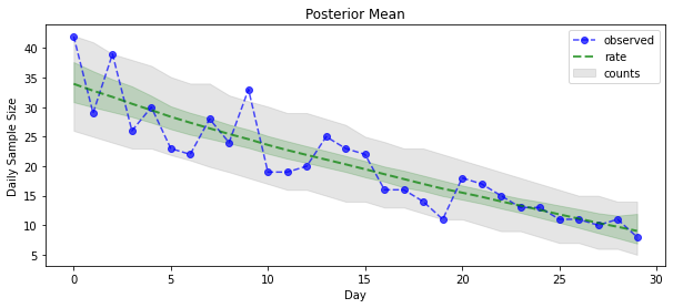
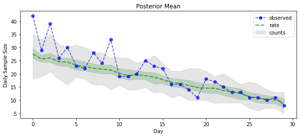
ようやく成果を見ることができます。ポワソン分布のレートに対する事後分布を見てみましょう!また、観測数に対して 80% の予測間隔もプロットし、この間隔に、実際に観測した数の約 80% が含まれているかを確認します。
param_samples = samples[:-1]
unconstrained_rate_samples = samples[-1][..., 0]
rate_samples = positive_bijector.forward(unconstrained_rate_samples)

plt.figure(figsize=(10, 4))
mean_lower, mean_upper = np.percentile(rate_samples, [10, 90], axis=0)
pred_lower, pred_upper = np.percentile(np.random.poisson(rate_samples),
                                       [10, 90], axis=0)

_ = plt.plot(observed_counts, color="blue", ls='--', marker='o', label='observed', alpha=0.7)
_ = plt.plot(np.mean(rate_samples, axis=0), label='rate', color="green", ls='dashed', lw=2, alpha=0.7)
_ = plt.fill_between(np.arange(0, 30), mean_lower, mean_upper, color='green', alpha=0.2)
_ = plt.fill_between(np.arange(0, 30), pred_lower, pred_upper, color='grey', label='counts', alpha=0.2)
plt.xlabel("Day")
plt.ylabel("Daily Sample Size")
plt.title("Posterior Mean")
plt.legend()
<matplotlib.legend.Legend at 0x7f93ffd35550>
予測
観測数を予測するために、標準 STS ツールを使用して、潜在レートに対する予測分布を構築し(STS は実際値データをモデル化するように設計されているため、制約なしの空間で)、サンプリングされた予測をポワソン型観測モデルに通します。
def sample_forecasted_counts(sts_model, posterior_latent_rates,
                             posterior_params, num_steps_forecast,
                             num_sampled_forecasts):

  # Forecast the future latent unconstrained rates, given the inferred latent
  # unconstrained rates and parameters.
  unconstrained_rates_forecast_dist = tfp.sts.forecast(sts_model,
    observed_time_series=unconstrained_rate_samples,
    parameter_samples=posterior_params,
    num_steps_forecast=num_steps_forecast)

  # Transform the forecast to positive-valued Poisson rates.
  rates_forecast_dist = tfd.TransformedDistribution(
      unconstrained_rates_forecast_dist,
      positive_bijector)

  # Sample from the forecast model following the chain rule:
  # P(counts) = P(counts | latent_rates)P(latent_rates)
  sampled_latent_rates = rates_forecast_dist.sample(num_sampled_forecasts)
  sampled_forecast_counts = tfd.Poisson(rate=sampled_latent_rates).sample()

  return sampled_forecast_counts, sampled_latent_rates

forecast_samples, rate_samples = sample_forecasted_counts(
   sts_model,
   posterior_latent_rates=unconstrained_rate_samples,
   posterior_params=param_samples,
   # Days to forecast:
   num_steps_forecast=30,
   num_sampled_forecasts=100)
forecast_samples = np.squeeze(forecast_samples)
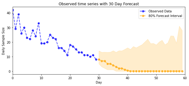
def plot_forecast_helper(data, forecast_samples, CI=90):
  """Plot the observed time series alongside the forecast."""
  plt.figure(figsize=(10, 4))
  forecast_median = np.median(forecast_samples, axis=0)

  num_steps = len(data)
  num_steps_forecast = forecast_median.shape[-1]

  plt.plot(np.arange(num_steps), data, lw=2, color='blue', linestyle='--', marker='o',
           label='Observed Data', alpha=0.7)

  forecast_steps = np.arange(num_steps, num_steps+num_steps_forecast)

  CI_interval = [(100 - CI)/2, 100 - (100 - CI)/2]
  lower, upper = np.percentile(forecast_samples, CI_interval, axis=0)

  plt.plot(forecast_steps, forecast_median, lw=2, ls='--', marker='o', color='orange',
           label=str(CI) + '% Forecast Interval', alpha=0.7)
  plt.fill_between(forecast_steps,
                   lower,
                   upper, color='orange', alpha=0.2)

  plt.xlim([0, num_steps+num_steps_forecast])
  ymin, ymax = min(np.min(forecast_samples), np.min(data)), max(np.max(forecast_samples), np.max(data))
  yrange = ymax-ymin
  plt.title("{}".format('Observed time series with ' + str(num_steps_forecast) + ' Day Forecast'))
  plt.xlabel('Day')
  plt.ylabel('Daily Sample Size')
  plt.legend()
plot_forecast_helper(observed_counts, forecast_samples, CI=80)
VI 推論
変分推論は、ここで行っている近似カウントのように(標準 STS モデルの一つの時系列のパラメータだけとは異なり)、全時系列を推論する場合に困難をきたす可能性があります。各時間ステップは隣接する時間ステップに相関しており、不確実性を過小評価する可能性があるため、変数に独立した事後分布があるという標準的な仮定はまったく間違っています。このため、全時系列に対する近似推論には、HMC がより適した選択肢である可能性があります。ただし、VI ははるかに高速であるため、モデルのプロトタイピングや、そのパフォーマンスが「十分に良好」であることが経験的に示される場合に役立つことがあります。
モデルを VI に適合するために、代替(サロゲート)事後分布を構築し、最適化します。
surrogate_posterior = tfp.experimental.vi.build_factored_surrogate_posterior(
    event_shape=pinned_model.event_shape,
    bijector=constraining_bijector)
# Allow external control of optimization to reduce test runtimes.
num_variational_steps = 1000 # @param { isTemplate: true}
num_variational_steps = int(num_variational_steps)

t0 = time.time()
losses = tfp.vi.fit_surrogate_posterior(pinned_model.unnormalized_log_prob,
                                        surrogate_posterior,
                                        optimizer=tf.optimizers.Adam(0.1),
                                        num_steps=num_variational_steps)
t1 = time.time()
print("Inference ran in {:.2f}s.".format(t1-t0))
Inference ran in 11.37s.
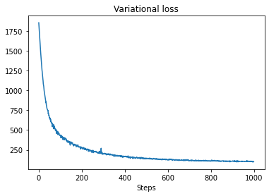
plt.plot(losses)
plt.title("Variational loss")
_ = plt.xlabel("Steps")
posterior_samples = surrogate_posterior.sample(50)
param_samples = posterior_samples[:-1]
unconstrained_rate_samples = posterior_samples[-1][..., 0]
rate_samples = positive_bijector.forward(unconstrained_rate_samples)

plt.figure(figsize=(10, 4))
mean_lower, mean_upper = np.percentile(rate_samples, [10, 90], axis=0)
pred_lower, pred_upper = np.percentile(
    np.random.poisson(rate_samples), [10, 90], axis=0)

_ = plt.plot(observed_counts, color='blue', ls='--', marker='o',
             label='observed', alpha=0.7)
_ = plt.plot(np.mean(rate_samples, axis=0), label='rate', color='green',
             ls='dashed', lw=2, alpha=0.7)
_ = plt.fill_between(
    np.arange(0, 30), mean_lower, mean_upper, color='green', alpha=0.2)
_ = plt.fill_between(np.arange(0, 30), pred_lower, pred_upper, color='grey',
    label='counts', alpha=0.2)
plt.xlabel('Day')
plt.ylabel('Daily Sample Size')
plt.title('Posterior Mean')
plt.legend()
<matplotlib.legend.Legend at 0x7f93ff4735c0>
forecast_samples, rate_samples = sample_forecasted_counts(
   sts_model,
   posterior_latent_rates=unconstrained_rate_samples,
   posterior_params=param_samples,
   # Days to forecast:
   num_steps_forecast=30,
   num_sampled_forecasts=100)
forecast_samples = np.squeeze(forecast_samples)
plot_forecast_helper(observed_counts, forecast_samples, CI=80)