このノートブックでは、いくつかの小さなスニペット(デモ)を介して TFP 0.11.0 で実現できることを紹介します。
| |
|
 GitHubでソースを表示 GitHubでソースを表示 |
Installs & imports
!pip3 install -U -q tensorflow==2.3.0 tensorflow_probability==0.11.0

import tensorflow as tf
import tensorflow_probability as tfp
assert '0.11' in tfp.__version__, tfp.__version__
assert '2.3' in tf.__version__, tf.__version__
tfd = tfp.distributions
tfb = tfp.bijectors
tfpk = tfp.math.psd_kernels

import matplotlib.pyplot as plt
import numpy as np
import scipy.interpolate
import IPython
import seaborn as sns
/usr/local/lib/python3.6/dist-packages/statsmodels/tools/_testing.py:19: FutureWarning: pandas.util.testing is deprecated. Use the functions in the public API at pandas.testing instead.
  import pandas.util.testing as tm
TFP は JAX で実行可能
注意: ナイトリービルドでは、これは tfp.substrates に移動されました。
import jax
from jax.config import config
config.update('jax_enable_x64', True)

def demo_jax():
  from tensorflow_probability.python.experimental.substrates import jax as tfp
  tfd = tfp.distributions
  tfb = tfp.bijectors

  @jax.jit
  def vmap_sample(seeds):
    d = tfb.Shift(2.)(tfb.Scale(2.)(tfd.Normal(0, 1)))
    return jax.vmap(lambda seed: d.sample(seed=seed))(seeds)

  def vmap_grad(seeds, sh, sc):
    d = lambda sh, sc: tfb.Shift(sh)(tfb.Scale(sc)(tfd.Normal(0, 1)))
    return jax.vmap(
        jax.grad(lambda sh, sc, samp: d(sh, sc).log_prob(samp),
                 argnums=(0,1,2)),
        in_axes=(None, None, 0))(sh, sc, vmap_sample(seeds))

  seed = jax.random.PRNGKey(123)
  seeds = jax.random.split(seed, 10)
  print('jit vmap sample:', vmap_sample(seeds))
  print('vmap grad:', vmap_grad(seeds, 2., 2.))

  @jax.jit
  def hmm_sample(seed):
    init, transition, obsv, sample = jax.random.split(seed, num=4)
    d = tfd.HiddenMarkovModel(
        initial_distribution=tfd.Categorical(logits=jax.random.uniform(init, [3]) + .1),
        transition_distribution=tfd.Categorical(logits=jax.random.uniform(transition, [3, 3]) + .1),
        observation_distribution=tfd.Normal(loc=jax.random.normal(obsv, [3]), scale=1.),
        num_steps=10)
    samps = d.sample(seed=sample)
    return samps, d.log_prob(samps)
  print('hmm:', hmm_sample(jax.random.PRNGKey(123)))

  @jax.jit
  def nuts(seed):
    return tfp.mcmc.sample_chain(
        num_results=10,
        num_burnin_steps=50,
        current_state=np.zeros([75]),
        kernel=tfp.mcmc.NoUTurnSampler(
            target_log_prob_fn=lambda x: -(x - .2)**2 / .05,
            step_size=.1),
        trace_fn=None,
        seed=seed)
  print('nuts:')
  plt.hist(nuts(seed=jax.random.PRNGKey(7)).reshape(-1), bins=20, density=True)

demo_jax()
/usr/local/lib/python3.6/dist-packages/jax/lib/xla_bridge.py:125: UserWarning: No GPU/TPU found, falling back to CPU.
  warnings.warn('No GPU/TPU found, falling back to CPU.')
jit vmap sample: [ 2.17746     2.6618252   3.427014   -0.80979496  5.87146     4.2002716
  1.2994273   1.2281269   3.5244293   4.1996603 ]
/usr/local/lib/python3.6/dist-packages/jax/numpy/lax_numpy.py:1531: FutureWarning: jax.numpy reductions won't accept lists and tuples in future versions, only scalars and ndarrays
  warnings.warn(msg, category=FutureWarning)
vmap grad: (DeviceArray([ 0.04436499,  0.1654563 ,  0.35675353, -0.70244873,
              0.96786499,  0.5500679 , -0.17514318, -0.19296828,
              0.38110733,  0.54991508], dtype=float64), DeviceArray([-0.4960635 , -0.44524843, -0.24545383,  0.48686844,
              1.37352526,  0.10514939, -0.43864973, -0.42552648,
             -0.20951441,  0.10481316], dtype=float64), DeviceArray([-0.04436499, -0.1654563 , -0.35675353,  0.7024487 ,
             -0.967865  , -0.5500679 ,  0.17514318,  0.19296828,
             -0.38110733, -0.5499151 ], dtype=float32))
hmm: (DeviceArray([-0.30260671, -0.38072154,  0.57980393, -0.30949971,
              1.22571819, -1.72733693, -1.13891736, -0.05021395,
              0.33300565, -0.31721795], dtype=float64), DeviceArray(-12.69673571, dtype=float64))
nuts:
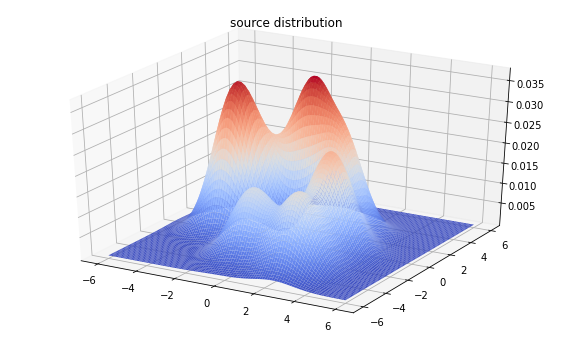
シーケンシャルモンテカルロによる推論(実験的)
nmodes = 7
loc_prior = tfd.MultivariateNormalDiag(loc=[0, 0], scale_diag=[2, 2])
mode_locs = loc_prior.sample(nmodes, seed=(0, 1))
logits_prior = tfd.Uniform()
mode_logits = logits_prior.sample(nmodes, seed=(0, 2))
make_mvn = lambda locs: tfd.MultivariateNormalDiag(
loc=locs, scale_diag=tf.ones_like(locs))
make_mixture = lambda locs, logits: tfd.MixtureSameFamily(
mixture_distribution=tfd.Categorical(logits=logits),
components_distribution=make_mvn(locs))
true_dist = make_mixture(mode_locs, mode_logits)
from mpl_toolkits import mplot3d
x = np.linspace(-6, 6, 100)
y = np.linspace(-6, 6, 100)
X, Y = np.asarray(np.meshgrid(x, y), dtype=np.float32)
Z = true_dist.prob(tf.stack([X, Y], axis=-1))
fig = plt.figure(figsize=(10, 6))
ax = plt.axes(projection='3d')
ax.plot_surface(
X, Y, Z, rstride=1, cstride=1, cmap='coolwarm', edgecolor='none')
plt.title('source distribution')
plt.show()
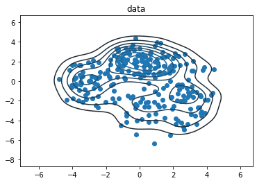
data_size = 256
samps = true_dist.sample(data_size, seed=(0, 3))
sns.kdeplot(*samps.numpy().T)
plt.scatter(*samps.numpy().T)
plt.title('data')
plt.show()
nparticles = 2048
seed = ()
(n_stage, final_state, final_kernel_results
  ) = tfp.experimental.mcmc.sample_sequential_monte_carlo(
      prior_log_prob_fn=lambda locs, logits: (
          tf.reduce_sum(loc_prior.log_prob(locs)) +
          tf.reduce_sum(logits_prior.log_prob(logits))),
      likelihood_log_prob_fn=lambda locs, logits: (
          tfd.Sample(make_mixture(locs, logits), data_size).log_prob(samps)),
      current_state=(loc_prior.sample([nparticles, nmodes + 2]),
                     logits_prior.sample([nparticles, nmodes + 2])),
)
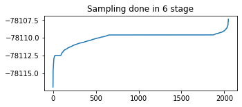
# Identify any issues with particle weight collapse.
plt.figure(figsize=(5,2))
plt.plot(tf.sort(final_kernel_results.particle_info.tempered_log_prob));
plt.title(f'Sampling done in {n_stage} stage');
sampled_distributions = tfd.MixtureSameFamily(
mixture_distribution=tfd.Categorical(
logits=final_kernel_results.particle_info.tempered_log_prob),
components_distribution=make_mixture(*final_state),
name='ensembled_posterior')
print(sampled_distributions)
Z = sampled_distributions.prob(tf.stack([X, Y], axis=-1))
fig = plt.figure(figsize=(10, 6))
ax = plt.axes(projection='3d')
ax.plot_surface(
X, Y, Z, rstride=1, cstride=1, cmap='coolwarm', edgecolor='none')
plt.title('Ensembled posterior probability density')
plt.show()
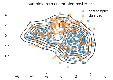
samps2 = sampled_distributions.sample(256, seed=(0, 4))
sns.kdeplot(*samps2.numpy().T)
# sns.kdeplot(*samps.numpy().T)
plt.scatter(*samps2.numpy().T, alpha=.5, label='new samples')
plt.scatter(*samps.numpy().T, alpha=.5, label='observed')
plt.legend()
plt.title('samples from ensembled posterior')
plt.show()
tfp.distributions.MixtureSameFamily("ensembled_posterior", batch_shape=[], event_shape=[2], dtype=float32)
球形分布: SphericalUniform(新規)、PowerSpherical(新規)、VonMisesFisher
plot_spherical
def plot_spherical(dist, nsamples):
  samples = dist.sample([nsamples], seed=123)
  probs = dist.prob(samples)
  samples = samples.numpy()
  probs = probs.numpy()
  # Show the dynamic range of the sample probabilities by re-scaling with min/max.
  minp, maxp = probs.min(), probs.max()
  ranged = np.float64(
      (probs - minp) / np.where(maxp - minp > 0, (maxp - minp), minp)) * .8 + .2

  data = list(map(list, samples))
  colors = map(plt.get_cmap('plasma'), ranged)
  colors = list(map(list, colors))

  js = """
    var scene = new THREE.Scene();
    var camera = new THREE.PerspectiveCamera( 75, 1.0, 0.1, 1000 );

    var renderer = new THREE.WebGLRenderer();
    renderer.setSize( 500, 500 );
    document.body.appendChild( renderer.domElement );

    var sphere_geom = new THREE.SphereBufferGeometry(1, 200, 200);
    var sphere_mat = new THREE.MeshBasicMaterial(
        {'opacity': 0.25, 'color': 0xFFFFFF, 'transparent': true});
    var sphere = new THREE.Mesh(sphere_geom, sphere_mat);
    sphere.position.set(0, 0, 0);
    scene.add(sphere);

    var points_data = %s;
    var points = [];
    for (var i = 0; i < points_data.length; i++) {
      points.push(new THREE.Vector3(
          points_data[i][0], points_data[i][1], points_data[i][2]));
    }

    var points_geom = new THREE.Geometry();
    points_geom.vertices = points;

    var colors_data = %s;
    var colors = [];
    for (var i = 0; i < colors_data.length; i++) {
      colors.push(new THREE.Color(
          colors_data[i][0], colors_data[i][1], colors_data[i][2]));
    }
    points_geom.colors = colors;
    var points_mat = new THREE.PointsMaterial({'size': 0.015});
    points_mat.vertexColors = THREE.VertexColors;
    var points = new THREE.Points(points_geom, points_mat);
    scene.add(points);

    camera.position.x = 0;
    camera.position.y = -2;
    camera.position.z = 2;
    camera.lookAt(new THREE.Vector3(0, 0, 0));

    controls = new THREE.TrackballControls(camera, renderer.domElement);
    controls.rotateSpeed = 1.0;
    controls.zoomSpeed = 1.2;
    controls.panSpeed = 0.8;
    controls.noZoom = false;
    controls.noPan = false;
    controls.staticMoving = false;
    controls.dynamicDampingFactor = 0.15;

    /*
    Keep the camera pointing the same direction it was before.  However,
    this does not generally have the same actual target as the original camera
    lookAt, only the same direction.  So when the user rotates the view it
    might not have the expected origin of rotation.
    */
    look_at = new THREE.Vector3(0, 0, -1);
    look_at.applyQuaternion(camera.quaternion).add(camera.position)
    controls.target = look_at;

    var LookAt = function(x, y, z) {
      camera.lookAt(new THREE.Vector3(x, y, z));
      controls.target.set(x, y, z);
    };
    LookAt(0, 0, 0);

    var animate = function () {
      requestAnimationFrame( animate );
      controls.update();
      renderer.render( scene, camera );
    };

    animate();
  """ % (repr(data), repr(colors))

  IPython.display.display_html("""
  <script type='text/javascript' src='https://ajax.googleapis.com/ajax/libs/threejs/r84/three.min.js'></script>
  <script type='text/javascript' src='https://cdn.rawgit.com/mrdoob/three.js/a1daef37/examples/js/controls/TrackballControls.js'></script>
  <script type='text/javascript'>
  %s
  </script>
  <b>Spin me!</b>
  """ % js, raw=True)
Visualizing tfd.SphericalUniform in 3 dimensions
nsamples = 2000
d = tfd.SphericalUniform(dimension=3)
plot_spherical(d, nsamples)
Visualizing tfd.PowerSpherical in 3 dimensions
concentration = 5.0
nsamples = 2000
d = tfd.PowerSpherical(
    mean_direction=tf.nn.l2_normalize(np.float64([1, 1, 1]), axis=-1),
    concentration=np.float64(concentration))
plot_spherical(d, nsamples)
Visualizing tfd.VonMisesFisher in 3 dimensions
concentration = 5.0
nsamples = 2000
vmf = tfp.distributions.VonMisesFisher(
    mean_direction=tf.nn.l2_normalize(np.float64([1, 1, 1]), axis=-1),
    concentration=np.float64(concentration))
plot_spherical(vmf, nsamples)
新しいバイジェクター
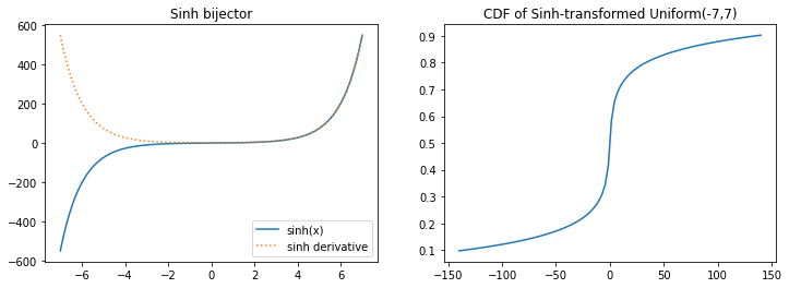
tfb.Sinh
plt.figure(figsize=(12, 4))
plt.subplot(121)
xs = np.linspace(-7, 7, 100)
plt.plot(xs, tfb.Sinh()(xs), label='sinh(x)')
plt.plot(xs, tf.math.exp(tfb.Sinh().forward_log_det_jacobian(xs, event_ndims=0)), ':', label='sinh derivative');
plt.legend()
plt.title('Sinh bijector')
plt.subplot(122)
xs *= 20
plt.plot(xs, tfb.Sinh()(tfd.Uniform(-7, 7)).cdf(xs))
plt.title('CDF of Sinh-transformed Uniform(-7,7)');
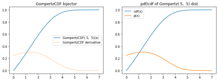
tfb.GompertzCDF
plt.figure(figsize=(12, 4))
plt.subplot(121)
xs = np.linspace(0, 7, 100).astype(np.float32)
b = tfb.GompertzCDF(.5, .5)
plt.plot(xs, b(xs), label='GompertzCDF(.5, .5)(x)')
plt.plot(xs, tf.math.exp(b.forward_log_det_jacobian(xs, event_ndims=0)), ':', label='GompertzCDF derivative');
plt.legend()
plt.title('GompertzCDF bijector')
plt.subplot(122)
d = tfb.Invert(b)(tfd.Uniform(0, 1))
plt.plot(xs, d.cdf(xs), label='cdf(x)')
plt.plot(xs, d.prob(xs), label='p(x)')
plt.legend()
plt.title('pdf/cdf of Gompertz(.5, .5) dist');
新しい分布
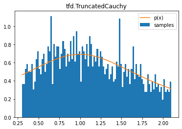
tfd.TruncatedCauchy
d = tfd.TruncatedCauchy(1, 1, .3, 2.1)
samples = tf.sort(d.sample(2000, seed=(0, 1)))
plt.hist(samples, bins=100, density=True, label='samples')
plt.plot(samples, d.prob(samples), label='p(x)')
plt.title('tfd.TruncatedCauchy')
plt.legend();
tfd.Bates (mean of n uniform samples)
plt.figure(figsize=(10, 5))
for i, n in enumerate((1, 3, 7, 13)):
  plt.subplot(221+i)
  d = tfd.Bates(total_count=n)
  samples = tf.sort(d.sample(2000, seed=(1, 2)))
  plt.hist(samples, bins=100, density=True, label='samples')
  plt.plot(samples, d.prob(samples), label='p(x)')
  plt.title(f'tfd.Bates | n={n}')
  plt.legend()
  plt.tight_layout()

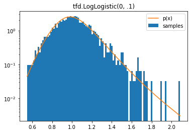
tfd.LogLogistic
d = tfd.LogLogistic(0, .1)
samples = tf.sort(d.sample(2000, seed=(2, 3)))
plt.hist(samples, bins=100, density=True, log=True, label='samples')
plt.plot(samples, d.prob(samples), label='p(x)')
plt.legend()
plt.title('tfd.LogLogistic(0, .1)');
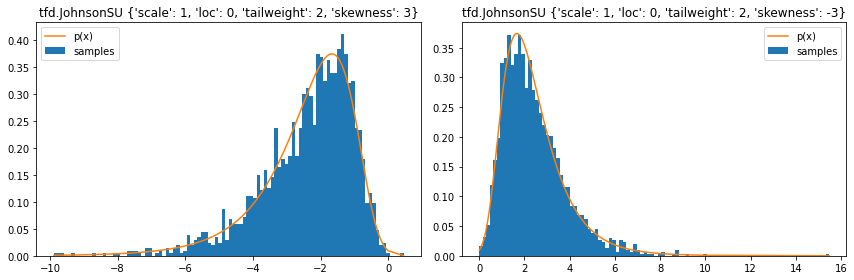
tfd.JohnsonSU
stats = ('loc', 'scale', 'tailweight', 'skewness')
plt.figure(figsize=(12, 4))
for i, d in enumerate([
    tfd.JohnsonSU(skewness=3, tailweight=2, loc=0, scale=1),
    tfd.JohnsonSU(skewness=-3, tailweight=2, loc=0, scale=1)]):
  plt.subplot(121+i)
  samples = tf.sort(d.sample(2000, seed=(2, 4)))
  plt.hist(samples, bins=100, density=True, label='samples')
  plt.plot(samples, d.prob(samples), label='p(x)')
  plt.legend()
  plt.title(f'tfd.JohnsonSU { {k: v for (k, v) in d.parameters.items() if k in stats} }')
  plt.tight_layout();
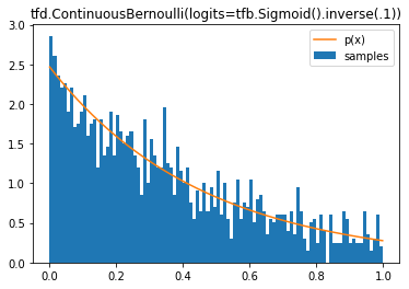
tfd.ContinuousBernoulli
d = tfd.ContinuousBernoulli(logits=tfb.Sigmoid().inverse(.1))
samples = tf.sort(d.sample(2000, seed=(2, 3)))
plt.hist(samples, bins=100, density=True, label='samples')
plt.plot(samples, d.prob(samples), label='p(x)')
plt.legend()
plt.title('tfd.ContinuousBernoulli(logits=tfb.Sigmoid().inverse(.1))');
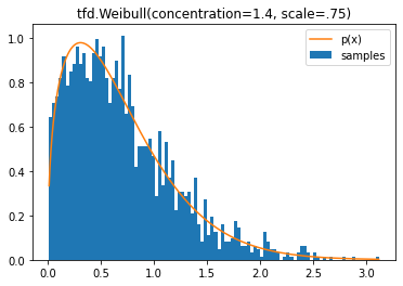
tfd.Weibull
d = tfd.Weibull(concentration=1.4, scale=.75)
samples = tf.sort(d.sample(2000, seed=(2, 3)))
plt.hist(samples, bins=100, density=True, label='samples')
plt.plot(samples, d.prob(samples), label='p(x)')
plt.legend()
plt.title('tfd.Weibull(concentration=1.4, scale=.75)');
JointDistribution*AutoBatched を使用した自動ベクトル化サンプリング
同時分布でバッチの次元を正しく合わせるには、これを推薦します。
このようなコードを記述したことはありますか?
data = tf.random.stateless_normal([7], seed=(1,2))

@tfd.JointDistributionCoroutine
def model():
  root = tfd.JointDistributionCoroutine.Root
  scale = yield root(tfd.Gamma(1, 1, name='scale'))
  yield tfd.Normal(tf.zeros_like(data), scale)

model.sample()
(<tf.Tensor: shape=(), dtype=float32, numpy=4.1253977>,
 <tf.Tensor: shape=(7,), dtype=float32, numpy=
 array([-2.814606  ,  0.81064916, -1.1025742 , -1.8684998 , -2.9547117 ,
        -0.19623983, -0.15587877], dtype=float32)>)
そして、非スカラーのサンプルを抽出する例外に遭遇したことはありますか?
print(model.sample(1), '\n  (^^ silent badness: the second value lacks a leading (1,) shape)')
print('sampling (3,) will break:')
import traceback
try:
  model.sample(3)
except ValueError as e:
  traceback.print_exc()
(<tf.Tensor: shape=(1,), dtype=float32, numpy=array([0.15810375], dtype=float32)>, <tf.Tensor: shape=(7,), dtype=float32, numpy=
array([-0.03214252,  0.15187298, -0.08423525, -0.03807954,  0.25466064,
       -0.14433853,  0.2543037 ], dtype=float32)>)
  (^^ silent badness: the second value lacks a leading (1,) shape)
sampling (3,) will break:
Traceback (most recent call last):
  File "/usr/local/lib/python3.6/dist-packages/tensorflow_probability/python/distributions/normal.py", line 243, in _parameter_control_dependencies
    self._batch_shape()
  File "/usr/local/lib/python3.6/dist-packages/tensorflow_probability/python/distributions/normal.py", line 176, in _batch_shape
    return tf.broadcast_static_shape(self.loc.shape, self.scale.shape)
  File "/usr/local/lib/python3.6/dist-packages/tensorflow/python/util/dispatch.py", line 201, in wrapper
    return target(*args, **kwargs)
  File "/usr/local/lib/python3.6/dist-packages/tensorflow/python/ops/array_ops.py", line 554, in broadcast_static_shape
    return common_shapes.broadcast_shape(shape_x, shape_y)
  File "/usr/local/lib/python3.6/dist-packages/tensorflow/python/framework/common_shapes.py", line 107, in broadcast_shape
    % (shape_x, shape_y))
ValueError: Incompatible shapes for broadcasting: (7,) and (3,)

During handling of the above exception, another exception occurred:

Traceback (most recent call last):
  File "<ipython-input-28-ab2fdd83415c>", line 4, in <module>
    model.sample(3)
  File "/usr/local/lib/python3.6/dist-packages/tensorflow_probability/python/distributions/distribution.py", line 939, in sample
    return self._call_sample_n(sample_shape, seed, name, **kwargs)
  File "/usr/local/lib/python3.6/dist-packages/tensorflow_probability/python/distributions/joint_distribution.py", line 532, in _call_sample_n
    **kwargs)
  File "/usr/local/lib/python3.6/dist-packages/tensorflow_probability/python/internal/distribution_util.py", line 1324, in _fn
    return fn(*args, **kwargs)
  File "/usr/local/lib/python3.6/dist-packages/tensorflow_probability/python/distributions/joint_distribution.py", line 414, in _sample_n
    **kwargs)
  File "/usr/local/lib/python3.6/dist-packages/tensorflow_probability/python/distributions/joint_distribution.py", line 451, in _call_flat_sample_distributions
    ds, xs = self._flat_sample_distributions(sample_shape, seed, value)
  File "/usr/local/lib/python3.6/dist-packages/tensorflow_probability/python/distributions/joint_distribution_coroutine.py", line 278, in _flat_sample_distributions
    d = gen.send(next_value)
  File "<ipython-input-19-d59a243cd9c8>", line 7, in model
    yield tfd.Normal(tf.zeros_like(data), scale)
  File "<decorator-gen-306>", line 2, in __init__
  File "/usr/local/lib/python3.6/dist-packages/tensorflow_probability/python/distributions/distribution.py", line 334, in wrapped_init
    default_init(self_, *args, **kwargs)
  File "/usr/local/lib/python3.6/dist-packages/tensorflow_probability/python/distributions/normal.py", line 148, in __init__
    name=name)
  File "/usr/local/lib/python3.6/dist-packages/tensorflow_probability/python/distributions/distribution.py", line 552, in __init__
    d for d in self._parameter_control_dependencies(is_init=True)
  File "/usr/local/lib/python3.6/dist-packages/tensorflow_probability/python/distributions/normal.py", line 248, in _parameter_control_dependencies
    self.loc.shape, self.scale.shape))
ValueError: Arguments `loc` and `scale` must have compatible shapes; loc.shape=(7,), scale.shape=(3,).
tfd.JointDistributionCoroutineAutoBatched などが使用できるようになりました
「スカラー」サンプリングルーチンを作成してから、任意のサンプル形状をドローします。
@tfd.JointDistributionCoroutineAutoBatched
def model_auto():
  scale = yield tfd.Gamma(1, 1, name='scale')
  yield tfd.Normal(tf.zeros_like(data), scale)

print(model_auto.sample(), '\n  (scalar sample)')
print(model_auto.sample(1), '\n  ((1,) sample)')
print(model_auto.sample(3), '\n  ((3,) sample)')
(<tf.Tensor: shape=(), dtype=float32, numpy=1.5234255>, <tf.Tensor: shape=(7,), dtype=float32, numpy=
array([-0.7177643 , -2.7825186 , -1.1250918 ,  0.57446253, -1.0755515 ,
        2.6673915 , -1.776087  ], dtype=float32)>)
  (scalar sample)
WARNING:tensorflow:Note that RandomUniformInt inside pfor op may not give same output as inside a sequential loop.
WARNING:tensorflow:Note that RandomUniformInt inside pfor op may not give same output as inside a sequential loop.
WARNING:tensorflow:Note that RandomStandardNormal inside pfor op may not give same output as inside a sequential loop.
WARNING:tensorflow:Note that RandomStandardNormal inside pfor op may not give same output as inside a sequential loop.
(<tf.Tensor: shape=(1,), dtype=float32, numpy=array([0.48698178], dtype=float32)>, <tf.Tensor: shape=(1, 7), dtype=float32, numpy=
array([[ 0.44244727, -0.548889  ,  0.29392514, -0.5249126 , -0.6618264 ,
         0.06925056, -0.32040703]], dtype=float32)>)
  ((1,) sample)
WARNING:tensorflow:Note that RandomUniformInt inside pfor op may not give same output as inside a sequential loop.
WARNING:tensorflow:Note that RandomUniformInt inside pfor op may not give same output as inside a sequential loop.
WARNING:tensorflow:Note that RandomStandardNormal inside pfor op may not give same output as inside a sequential loop.
(<tf.Tensor: shape=(3,), dtype=float32, numpy=array([0.5501703, 1.9277483, 2.7804365], dtype=float32)>, <tf.Tensor: shape=(3, 7), dtype=float32, numpy=
array([[-1.1568309 ,  0.02062727,  0.04918252, -0.08978909,  0.6446161 ,
        -0.16725235, -0.27897784],
       [-2.9246418 , -1.2733852 ,  1.0071639 , -0.4655921 , -4.1095695 ,
         0.1298227 ,  3.0307395 ],
       [-2.7411313 ,  1.6211014 , -1.600051  , -1.4009917 ,  4.081262  ,
         1.7097493 ,  2.8525631 ]], dtype=float32)>)
  ((3,) sample)
eager でも再現性のあるサンプリング
tf.random.set_seed(123)
print('Stateful sampling:\t\t',
      tfd.Normal(0, 1).sample(seed=234),
      'then',
      tfd.Normal(0, 1).sample(seed=234))

# Why are they different?
# TF samplers are stateful by default (TF maintains is a global PRNG).
# How to get reproducible results in eager mode?
tf.random.set_seed(123)
print('Stateful sampling (set_seed):\t',
      tfd.Normal(0, 1).sample(seed=234))

# And what about tf.function?
@tf.function
def sample_normal():
  return tfd.Normal(0, 1).sample(seed=234)
tf.random.set_seed(123)
print('tf.function:\t\t', sample_normal(), 'vs', sample_normal())
tf.random.set_seed(123)
print('tf.function (set_seed):\t', sample_normal())

# Using a Tensor seed (or a tuple, which TFP will convert to a tensor) induces
# TFP behavior analagous to the tf.random.stateless_* ops. This sampling
# is fully deterministic.
print('Stateless sampling (tuple):\t\t',
      tfd.Normal(0, 1).sample(seed=(1, 23)))
print('Stateless sampling (tensor):\t\t',
      tfd.Normal(0, 1).sample(seed=tf.constant([1, 23], dtype=tf.int32)))
# Even in tf.function
@tf.function
def sample_normal():
  return tfd.Normal(0, 1).sample(seed=(1, 23))
print('Stateless sampling (tf.function):\t', sample_normal())

# And independent of global seeds.
tf.random.set_seed(321)
print('Stateless sampling (ignores set_seed):\t', sample_normal())
Stateful sampling:         tf.Tensor(0.54054874, shape=(), dtype=float32) then tf.Tensor(-1.5518123, shape=(), dtype=float32)
Stateful sampling (set_seed):  tf.Tensor(0.54054874, shape=(), dtype=float32)
tf.function:       tf.Tensor(0.54054874, shape=(), dtype=float32) vs tf.Tensor(-1.5518123, shape=(), dtype=float32)
tf.function (set_seed):    tf.Tensor(0.54054874, shape=(), dtype=float32)
Stateless sampling (tuple):        tf.Tensor(-0.36107817, shape=(), dtype=float32)
Stateless sampling (tensor):       tf.Tensor(-0.36107817, shape=(), dtype=float32)
Stateless sampling (tf.function):  tf.Tensor(-0.36107817, shape=(), dtype=float32)
Stateless sampling (ignores set_seed):     tf.Tensor(-0.36107817, shape=(), dtype=float32)
同様に、tfp.mcmc.sample_chain はステートレスシードを受け入れるようになりました
これは基礎となるカーネルに渡され、ランダムな提案を行う場合は、one_step への seed 引数を受け入れるように更新する必要があります。(組み込みのカーネルはすでに更新されています。)
kernel = tfp.mcmc.HamiltonianMonteCarlo(lambda x: -(x - .2)**2,
                                        step_size=1.,
                                        num_leapfrog_steps=2)
print_n_lines = lambda x, n: print('\n'.join(repr(x).split('\n')[:n] + ['...']))
print_n_lines(
    tfp.mcmc.sample_chain(
        num_results=5,
        num_burnin_steps=100,
        current_state=tf.zeros([3]),
        kernel=kernel,
        trace_fn=lambda state, kr: kr,
        seed=(1, 2)),
    17)
print('And again (reproducibly)...')
print_n_lines(
    tfp.mcmc.sample_chain(
        num_results=5,
        num_burnin_steps=100,
        current_state=tf.zeros([3]),
        kernel=kernel,
        trace_fn=lambda state, kr: kr,
        seed=(1, 2)),
    17)
StatesAndTrace(
  all_states=<tf.Tensor: shape=(5, 3), dtype=float32, numpy=
    array([[ 4.0000078e-01,  3.9999962e-01,  3.9999855e-01],
           [-8.3446503e-07,  3.5762787e-07,  1.5497208e-06],
           [ 4.0000081e-01,  3.9999965e-01,  3.9999846e-01],
           [-8.3446503e-07,  4.7683716e-07,  1.5497208e-06],
           [ 4.0000087e-01,  3.9999962e-01,  3.9999843e-01]], dtype=float32)>,
  trace=MetropolisHastingsKernelResults(
      accepted_results=UncalibratedHamiltonianMonteCarloKernelResults(
          log_acceptance_correction=<tf.Tensor: shape=(5, 3), dtype=float32, numpy=
            array([[ 0.0000000e+00, -2.9802322e-08,  0.0000000e+00],
                   [ 5.9604645e-08,  1.1175871e-08,  1.1920929e-07],
                   [-2.9802322e-08, -2.7939677e-09,  2.7939677e-09],
                   [ 0.0000000e+00,  0.0000000e+00, -5.9604645e-08],
                   [ 1.4901161e-08, -1.7881393e-07,  0.0000000e+00]], dtype=float32)>,
          target_log_prob=<tf.Tensor: shape=(5, 3), dtype=float32, numpy=
            array([[-0.04000031, -0.03999985, -0.03999942],
...
And again (reproducibly)...
StatesAndTrace(
  all_states=<tf.Tensor: shape=(5, 3), dtype=float32, numpy=
    array([[ 4.0000078e-01,  3.9999962e-01,  3.9999855e-01],
           [-8.3446503e-07,  3.5762787e-07,  1.5497208e-06],
           [ 4.0000081e-01,  3.9999965e-01,  3.9999846e-01],
           [-8.3446503e-07,  4.7683716e-07,  1.5497208e-06],
           [ 4.0000087e-01,  3.9999962e-01,  3.9999843e-01]], dtype=float32)>,
  trace=MetropolisHastingsKernelResults(
      accepted_results=UncalibratedHamiltonianMonteCarloKernelResults(
          log_acceptance_correction=<tf.Tensor: shape=(5, 3), dtype=float32, numpy=
            array([[ 0.0000000e+00, -2.9802322e-08,  0.0000000e+00],
                   [ 5.9604645e-08,  1.1175871e-08,  1.1920929e-07],
                   [-2.9802322e-08, -2.7939677e-09,  2.7939677e-09],
                   [ 0.0000000e+00,  0.0000000e+00, -5.9604645e-08],
                   [ 1.4901161e-08, -1.7881393e-07,  0.0000000e+00]], dtype=float32)>,
          target_log_prob=<tf.Tensor: shape=(5, 3), dtype=float32, numpy=
            array([[-0.04000031, -0.03999985, -0.03999942],
...
MCMC カーネルの結果を出力する
tfp.mcmc.RandomWalkMetropolis(tfd.Uniform(0, 10).log_prob).bootstrap_results(1.)
MetropolisHastingsKernelResults(
  accepted_results=UncalibratedRandomWalkResults(
      log_acceptance_correction=<tf.Tensor: shape=(), dtype=float32, numpy=0.0>,
      target_log_prob=<tf.Tensor: shape=(), dtype=float32, numpy=-2.3025851>,
      seed=[]
    ),
  is_accepted=<tf.Tensor: shape=(), dtype=bool, numpy=True>,
  log_accept_ratio=<tf.Tensor: shape=(), dtype=float32, numpy=0.0>,
  proposed_state=1.0,
  proposed_results=UncalibratedRandomWalkResults(
      log_acceptance_correction=<tf.Tensor: shape=(), dtype=float32, numpy=0.0>,
      target_log_prob=<tf.Tensor: shape=(), dtype=float32, numpy=-2.3025851>,
      seed=<tf.Tensor: shape=(2,), dtype=int32, numpy=array([0, 0], dtype=int32)>
    ),
  extra=[],
  seed=<tf.Tensor: shape=(2,), dtype=int32, numpy=array([0, 0], dtype=int32)>
)
CompositeTensor (実験的)
tf.function のトレースを省きます。tf.function から分布を返します。
@tf.function
def get_mean(d):
  return d.mean()

print(get_mean(tfp.experimental.as_composite(tfd.BetaBinomial(100., 2., 7.))))

@tf.function
def returns_dist(logits):
  return tfp.experimental.as_composite(tfd.Binomial(10., logits=logits))

print(returns_dist(tf.constant(0.)),
      returns_dist(tf.constant(0.)).sample(seed=(2, 3)))
tf.Tensor(22.222221, shape=(), dtype=float32)
tfp.distributions.BinomialCT("Binomial", batch_shape=[], event_shape=[], dtype=float32) tf.Tensor(5.0, shape=(), dtype=float32)
ご存知ですか: バッチスライス分布
def demo_batch_slice():
  d = tfd.Normal(
      loc=tf.random.stateless_normal([100, 20, 3], seed=(1,2)),
      scale=1.)
  print(d, '\n  (original dist)')
  print(d[0], '\n  (0th element of the first batch dimension)')
  print(d[::2, ..., 1], '\n  (every other element of first dim  x  middle element of final dim)\n')

  d = tfd.Dirichlet(
      concentration=tf.random.stateless_uniform([100, 20, 3, 7], seed=(1,2)))
  print(d, '\n  (original dist)')
  print(d[:, 0], '\n  (0th element of the second dimension)')
  print(d[::2, ..., 1], '\n  (every other element of first dim  x  middle element of final dim)')
demo_batch_slice()
tfp.distributions.Normal("Normal", batch_shape=[100, 20, 3], event_shape=[], dtype=float32)
  (original dist)
tfp.distributions.Normal("Normal", batch_shape=[20, 3], event_shape=[], dtype=float32)
  (0th element of the first batch dimension)
tfp.distributions.Normal("Normal", batch_shape=[50, 20], event_shape=[], dtype=float32)
  (every other element of first dim  x  middle element of final dim)

tfp.distributions.Dirichlet("Dirichlet", batch_shape=[100, 20, 3], event_shape=[7], dtype=float32)
  (original dist)
tfp.distributions.Dirichlet("Dirichlet", batch_shape=[100, 3], event_shape=[7], dtype=float32)
  (0th element of the second dimension)
tfp.distributions.Dirichlet("Dirichlet", batch_shape=[50, 20], event_shape=[7], dtype=float32)
  (every other element of first dim  x  middle element of final dim)
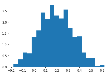
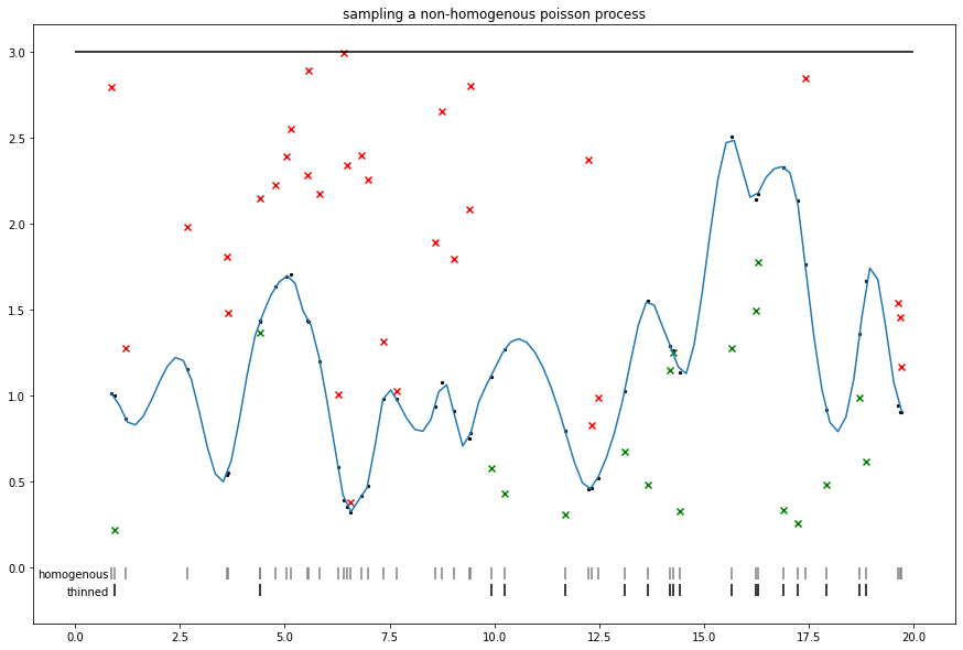
ランダムノベルティ:シグモイドコックス(不均一ポアソン)過程のサンプリング
Adams et al. で提案されている細線化を使用します。
同様の細線化アプローチは、強度の上限を使用して、不均一なイベントをサンプリングする非可逆 MCMC に対するいくつかのアプローチに関連していることに注意してください(例:ジグザグや往復する粒子サンプラー)。
def sigmoidal_cox_process():
  V = 20.
  lam0 = 3.
  n_homog = tfd.Poisson(V * lam0).sample(seed=(0, 1))
  homog_locs = tf.sort(tfd.Uniform(0., V).sample(n_homog, seed=(0, 2)))
  homog_intensities = tfd.GaussianProcess(
      tfpk.MaternThreeHalves(),
      index_points=homog_locs[:, tf.newaxis]).sample(seed=(0, 3))

  plt.figure(figsize=(15,10))
  plt.title('sampling a non-homogenous poisson process')
  plt.hlines(lam0, xmin=0., xmax=V)

  sigm_int = tf.math.sigmoid(homog_intensities) * lam0

  sp = scipy.interpolate.make_interp_spline(homog_locs, sigm_int)
  xs = np.linspace(homog_locs[0], homog_locs[-1], 100)
  ys = scipy.interpolate.splev(xs, sp)
  plt.plot(xs, ys)

  plt.scatter(homog_locs, sigm_int, s=5., c='black')

  unif = tfd.Uniform(0, lam0).sample(n_homog)
  plt.scatter(homog_locs, tf.where(unif < sigm_int, np.nan, unif), c='r', marker='x')
  plt.scatter(homog_locs, tf.where(unif > sigm_int, np.nan, unif), c='g', marker='x')

  plt.vlines(homog_locs, 0, -.07, colors='gray', )
  plt.text(.8, -.06, 'homogenous', dict(fontsize='medium'), horizontalalignment='right')

  nonhomog_locs = tf.gather(homog_locs, tf.where(unif < sigm_int))
  plt.vlines(nonhomog_locs, -.1, -.17, colors='black')
  plt.text(.8, -.16, 'thinned', dict(fontsize='medium'), horizontalalignment='right')
  plt.show()

sigmoidal_cox_process()
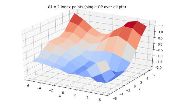
ご存知ですか: GP のバッチ
ガウス過程は、関数全体の分布です。ここでは、カーネルと一連のインデックスポイントによってパラメータ化し、バッチ処理の動作の一部を紹介します。
(TFP は GP 回帰モデルもサポートします。このモデルでは、観測されたインデックスポイントでの観測により、一連のインデックスポイントの関数の事後分布が決定されます。tfd.GaussianProcessRegressionModel を参照してください。)
from mpl_toolkits import mplot3d
x = np.linspace(-6, 6, 9)
y = np.linspace(-6, 6, 9)
X, Y = np.asarray(np.meshgrid(x, y), dtype=np.float32)
print('We can set up a single GP over many examples of 2d feature')
gp = tfd.GaussianProcess(
tfpk.ExponentiatedQuadratic(length_scale=3., feature_ndims=1),
index_points=tf.reshape(tf.stack([X, Y], axis=-1), (-1, 2)),
jitter=1e-3)
print(gp)
Z = tf.reshape(gp.sample(seed=(0,3)), X.shape)
fig = plt.figure(figsize=(10, 6))
ax = plt.axes(projection='3d')
ax.plot_surface(
X, Y, Z, rstride=1, cstride=1, cmap='coolwarm', edgecolor='none');
ax.set_xlabel('x');ax.set_ylabel('y');
ax.set_title('81 x 2 index points (single GP over all pts)')
plt.show()
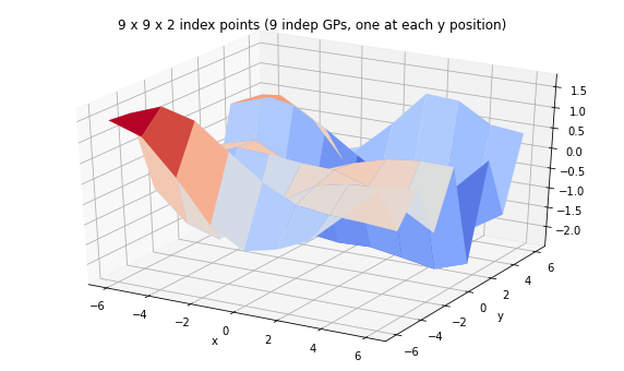
print('We can have a batch of independent GPs with their own sets of index points.')
batch_gp = tfd.GaussianProcess(
tfpk.ExponentiatedQuadratic(length_scale=3., feature_ndims=1),
index_points=tf.stack([X, Y], axis=-1),
jitter=1e-3)
print(batch_gp)
Z_batch = batch_gp.sample(seed=(5,7))
fig = plt.figure(figsize=(10, 6))
ax = plt.axes(projection='3d')
ax.plot_surface(
X, Y, Z_batch, rstride=1, cstride=1, cmap='coolwarm', edgecolor='none');
ax.set_xlabel('x');ax.set_ylabel('y');
ax.set_title('9 x 9 x 2 index points (9 indep GPs, one at each y position)');
plt.show()
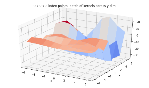
print('We can also have a corresponding batch of kernels.')
kernel = tfpk.ExponentiatedQuadratic(length_scale=3.,
amplitude=tf.linspace(1., 20., 9),
feature_ndims=1)
print(kernel)
batch_gp_kernel = tfd.GaussianProcess(
kernel,
index_points=tf.stack([X, Y], axis=-1),
jitter=1e-3)
print(batch_gp_kernel)
Z_batch_kernel = batch_gp_kernel.sample(seed=(5,7))
fig = plt.figure(figsize=(10, 6))
ax = plt.axes(projection='3d')
ax.plot_surface(
X, Y, Z_batch_kernel, rstride=1, cstride=1, cmap='coolwarm', edgecolor='none');
ax.set_xlabel('x');ax.set_ylabel('y');
ax.set_title('9 x 9 x 2 index points, batch of kernels across y dim');
We can set up a single GP over many examples of 2d feature
tfp.distributions.GaussianProcess("GaussianProcess", batch_shape=[], event_shape=[81], dtype=float32)
We can also have a corresponding batch of kernels.
tfp.math.psd_kernels.ExponentiatedQuadratic("ExponentiatedQuadratic", batch_shape=(9,), feature_ndims=1, dtype=float32)
tfp.distributions.GaussianProcess("GaussianProcess", batch_shape=[9], event_shape=[9], dtype=float32)
We can also have a corresponding batch of kernels.
tfp.math.psd_kernels.ExponentiatedQuadratic("ExponentiatedQuadratic", batch_shape=(9,), feature_ndims=1, dtype=float32)
tfp.distributions.GaussianProcess("GaussianProcess", batch_shape=[9], event_shape=[9], dtype=float32)