
<style> td { text-align: center; } th { text-align: center; } </style>
 在 GitHub 上查看源代码 在 GitHub 上查看源代码 |
|
给定一个类似以下示例的图像,我们的目标是生成一个类似“一名正在冲浪的冲浪者”的描述。
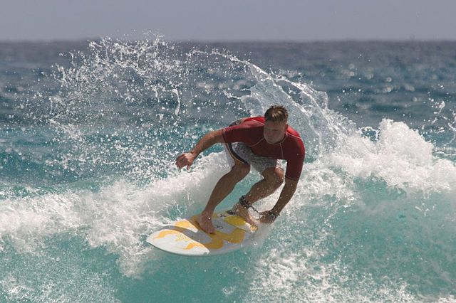 |
| 一个冲浪的人,来自 Wikimedia |
|---|
此处使用的模型架构的灵感来自 Show, Attend and Tell: Neural Image Caption Generation with Visual Attention,但已更新为使用 2 层 Transformer 解码器。要充分利用本教程,您应该对文本生成、seq2seq 模型和注意力或 Transformer 有一定的经验。
本教程中构建的模型架构如下所示。从图像中提取特征,并传递到 Transformer 解码器的交叉注意力层。
| 模型架构 |
|---|
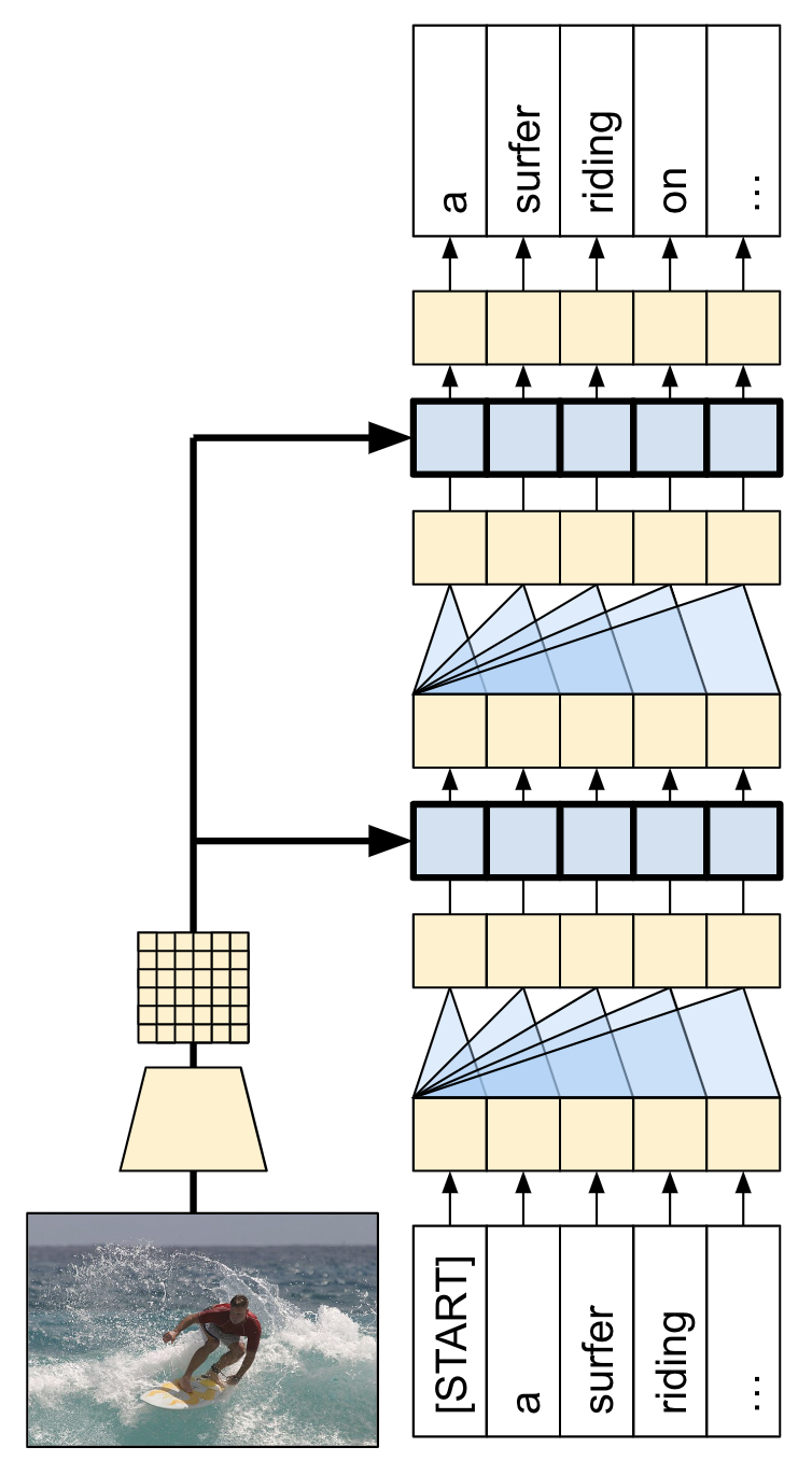 |
Transformer 解码器主要由注意力层构建。它使用自注意力处理正在生成的序列,并使用交叉注意力处理图像。
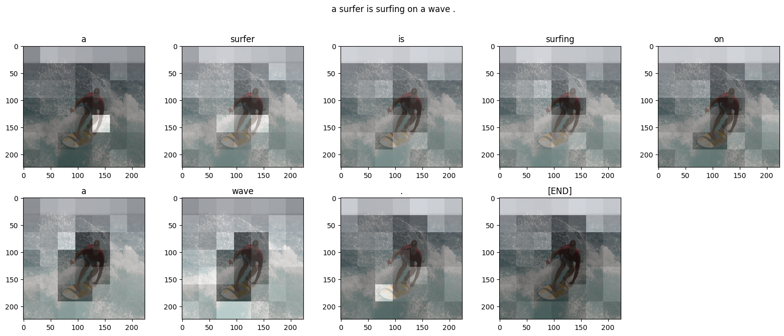
通过检查交叉注意力层的注意力权重,您将看到模型在生成单词时正在查看图像的哪些部分。
此笔记本是一个端到端示例。当您运行此笔记本时,它会下载数据集、提取和缓存图像特征,并训练解码器模型。随后,它会使用该模型在新的图像上生成描述。
安装
apt install --allow-change-held-packages libcudnn8=8.1.0.77-1+cuda11.2pip uninstall -y tensorflow estimator keraspip install -U tensorflow_text tensorflow tensorflow_datasetspip install einops本教程使用大量导入,主要用于加载数据集。
import concurrent.futures
import collections
import dataclasses
import hashlib
import itertools
import json
import math
import os
import pathlib
import random
import re
import string
import time
import urllib.request

import einops
import matplotlib.pyplot as plt
import numpy as np
import pandas as pd
from PIL import Image
import requests
import tqdm

import tensorflow as tf
import tensorflow_hub as hub
import tensorflow_text as text
import tensorflow_datasets as tfds
[可选] 数据处理
本部分下载描述数据集并为训练做准备。它将输入文本词例化,并缓存通过预训练的特征提取程序模型运行所有图像的结果。理解本部分中的所有内容并不是非常重要。
选择数据集
本教程旨在提供数据集的选择。Flickr8k 或 Conceptual Captions 数据集的一小部分。这两个数据集需要从头开始下载和转换,但是将教程转换为使用 TensorFlow 数据集中可用的描述数据集(Coco Captions 和完整的 Conceptual Captions)并不难。
Flickr8k
def flickr8k(path='flickr8k'):
  path = pathlib.Path(path)

  if len(list(path.rglob('*'))) < 16197:
    tf.keras.utils.get_file(
        origin='https://github.com/jbrownlee/Datasets/releases/download/Flickr8k/Flickr8k_Dataset.zip',
        cache_dir='.',
        cache_subdir=path,
        extract=True)
    tf.keras.utils.get_file(
        origin='https://github.com/jbrownlee/Datasets/releases/download/Flickr8k/Flickr8k_text.zip',
        cache_dir='.',
        cache_subdir=path,
        extract=True)

  captions = (path/"Flickr8k.token.txt").read_text().splitlines()
  captions = (line.split('\t') for line in captions)
  captions = ((fname.split('#')[0], caption) for (fname, caption) in captions)

  cap_dict = collections.defaultdict(list)
  for fname, cap in captions:
    cap_dict[fname].append(cap)

  train_files = (path/'Flickr_8k.trainImages.txt').read_text().splitlines()
  train_captions = [(str(path/'Flicker8k_Dataset'/fname), cap_dict[fname]) for fname in train_files]

  test_files = (path/'Flickr_8k.testImages.txt').read_text().splitlines()
  test_captions = [(str(path/'Flicker8k_Dataset'/fname), cap_dict[fname]) for fname in test_files]

  train_ds = tf.data.experimental.from_list(train_captions)
  test_ds = tf.data.experimental.from_list(test_captions)

  return train_ds, test_ds
Conceptual Captions
def conceptual_captions(*, data_dir="conceptual_captions", num_train, num_val):
  def iter_index(index_path):
    with open(index_path) as f:
      for line in f:
        caption, url = line.strip().split('\t')
        yield caption, url

  def download_image_urls(data_dir, urls):
    ex = concurrent.futures.ThreadPoolExecutor(max_workers=100)
    def save_image(url):
      hash = hashlib.sha1(url.encode())
      # Name the files after the hash of the URL.
      file_path = data_dir/f'{hash.hexdigest()}.jpeg'
      if file_path.exists():
        # Only download each file once.
        return file_path

      try:
        result = requests.get(url, timeout=5)
      except Exception:
        file_path = None
      else:
        file_path.write_bytes(result.content)
      return file_path

    result = []
    out_paths = ex.map(save_image, urls)
    for file_path in tqdm.tqdm(out_paths, total=len(urls)):
      result.append(file_path)

    return result

  def ds_from_index_file(index_path, data_dir, count):
    data_dir.mkdir(exist_ok=True)
    index = list(itertools.islice(iter_index(index_path), count))
    captions = [caption for caption, url in index]
    urls = [url for caption, url in index]

    paths = download_image_urls(data_dir, urls)

    new_captions = []
    new_paths = []
    for cap, path in zip(captions, paths):
      if path is None:
        # Download failed, so skip this pair.
        continue
      new_captions.append(cap)
      new_paths.append(path)

    new_paths = [str(p) for p in new_paths]

    ds = tf.data.Dataset.from_tensor_slices((new_paths, new_captions))
    ds = ds.map(lambda path,cap: (path, cap[tf.newaxis])) # 1 caption per image
    return ds

  data_dir = pathlib.Path(data_dir)
  train_index_path = tf.keras.utils.get_file(
    origin='https://storage.googleapis.com/gcc-data/Train/GCC-training.tsv',
    cache_subdir=data_dir,
    cache_dir='.')

  val_index_path = tf.keras.utils.get_file(
    origin='https://storage.googleapis.com/gcc-data/Validation/GCC-1.1.0-Validation.tsv',
    cache_subdir=data_dir,
    cache_dir='.')

  train_raw = ds_from_index_file(train_index_path, data_dir=data_dir/'train', count=num_train)
  test_raw = ds_from_index_file(val_index_path, data_dir=data_dir/'val', count=num_val)

  return train_raw, test_raw
下载数据集
Flickr8k 是一个不错的选择,因为它每个图像包含 5 个描述,下载更少,数据更多。
choose = 'flickr8k'

if choose == 'flickr8k':
  train_raw, test_raw = flickr8k()
else:
  train_raw, test_raw = conceptual_captions(num_train=10000, num_val=5000)
上面两个数据集的加载程序都返回包含 (image_path, captions) 对的 tf.data.Dataset。Flickr8k 数据集每个图像包含 5 个描述,而 Conceptual Captions 有 1 个:
train_raw.element_spec
for ex_path, ex_captions in train_raw.take(1):
  print(ex_path)
  print(ex_captions)
图像特征提取程序
您将使用图像模型(在 imagenet 上预训练)从每个图像中提取特征。该模型被训练为图像分类器,但设置 include_top=False 会返回没有最终分类层的模型,因此您可以使用特征映射的最后一层:
IMAGE_SHAPE=(224, 224, 3)
mobilenet = tf.keras.applications.MobileNetV3Small(
    input_shape=IMAGE_SHAPE,
    include_top=False,
    include_preprocessing=True)
mobilenet.trainable=False
下面是一个加载图像并为模型调整大小的函数:
def load_image(image_path):
    img = tf.io.read_file(image_path)
    img = tf.io.decode_jpeg(img, channels=3)
    img = tf.image.resize(img, IMAGE_SHAPE[:-1])
    return img
该模型为输入批次中的每个图像返回一个特征映射:
test_img_batch = load_image(ex_path)[tf.newaxis, :]

print(test_img_batch.shape)
print(mobilenet(test_img_batch).shape)
设置文本分词器/向量化程序
使用 TextVectorization 层将文本描述转换为整数序列,步骤如下:
- 使用 adapt 迭代所有描述,将描述拆分为字词,并计算最热门字词的词汇表。
- 通过将每个字词映射到它在词汇表中的索引对所有描述进行词例化。所有输出序列将被填充到长度 50。
- 创建字词到索引和索引到字词的映射以显示结果。
def standardize(s):
  s = tf.strings.lower(s)
  s = tf.strings.regex_replace(s, f'[{re.escape(string.punctuation)}]', '')
  s = tf.strings.join(['[START]', s, '[END]'], separator=' ')
  return s
# Use the top 5000 words for a vocabulary.
vocabulary_size = 5000
tokenizer = tf.keras.layers.TextVectorization(
    max_tokens=vocabulary_size,
    standardize=standardize,
    ragged=True)
# Learn the vocabulary from the caption data.
tokenizer.adapt(train_raw.map(lambda fp,txt: txt).unbatch().batch(1024))
tokenizer.get_vocabulary()[:10]
t = tokenizer([['a cat in a hat'], ['a robot dog']])
t
# Create mappings for words to indices and indices to words.
word_to_index = tf.keras.layers.StringLookup(
    mask_token="",
    vocabulary=tokenizer.get_vocabulary())
index_to_word = tf.keras.layers.StringLookup(
    mask_token="",
    vocabulary=tokenizer.get_vocabulary(),
    invert=True)
w = index_to_word(t)
w.to_list()
tf.strings.reduce_join(w, separator=' ', axis=-1).numpy()
准备数据集
train_raw 和 test_raw 数据集包含一对多 (image, captions) 对。
此函数将复制图像,因此描述中有 1:1 的图像:
def match_shapes(images, captions):
  caption_shape = einops.parse_shape(captions, 'b c')
  captions = einops.rearrange(captions, 'b c -> (b c)')
  images = einops.repeat(
      images, 'b ... -> (b c) ...',
      c = caption_shape['c'])
  return images, captions
for ex_paths, ex_captions in train_raw.batch(32).take(1):
  break

print('image paths:', ex_paths.shape)
print('captions:', ex_captions.shape)
print()

ex_paths, ex_captions = match_shapes(images=ex_paths, captions=ex_captions)

print('image_paths:', ex_paths.shape)
print('captions:', ex_captions.shape)
为了与 keras 训练兼容,数据集应包含 (inputs, labels) 对。对于文本生成,词例既是输入又是标签,且移动了一步。此函数会将 (images, texts) 对转换为 ((images, input_tokens), label_tokens) 对:
def prepare_txt(imgs, txts):
  tokens = tokenizer(txts)

  input_tokens = tokens[..., :-1]
  label_tokens = tokens[..., 1:]
  return (imgs, input_tokens), label_tokens
此函数会将运算添加到数据集。步骤如下:
- 加载图像(忽略加载失败的图像)。
- 复制图像以匹配描述的数量。
- 对
image, caption对执行重排和重新批处理。 - 将文本词例化,移动词例并添加
label_tokens。 - 将文本从
RaggedTensor表示转换为填充的密集Tensor表示。
def prepare_dataset(ds, tokenizer, batch_size=32, shuffle_buffer=1000):
  # Load the images and make batches.
  ds = (ds
        .shuffle(10000)
        .map(lambda path, caption: (load_image(path), caption))
        .apply(tf.data.experimental.ignore_errors())
        .batch(batch_size))

  def to_tensor(inputs, labels):
    (images, in_tok), out_tok = inputs, labels
    return (images, in_tok.to_tensor()), out_tok.to_tensor()

  return (ds
          .map(match_shapes, tf.data.AUTOTUNE)
          .unbatch()
          .shuffle(shuffle_buffer)
          .batch(batch_size)
          .map(prepare_txt, tf.data.AUTOTUNE)
          .map(to_tensor, tf.data.AUTOTUNE)
          )
您可以在模型中安装特征提取程序并在数据集上进行训练,如下所示:
train_ds = prepare_dataset(train_raw, tokenizer)
train_ds.element_spec
test_ds = prepare_dataset(test_raw, tokenizer)
test_ds.element_spec
[可选] 缓存图像特征
由于图像特征提取程序没有更改,并且本教程没有使用图像增强,可以缓存图像特征。文本词例化也是如此。在训练和验证期间,每个周期都可以重新获得设置缓存所需的时间。下面的代码定义了两个函数 (save_dataset 和 load_dataset):
def save_dataset(ds, save_path, image_model, tokenizer, shards=10, batch_size=32):
  # Load the images and make batches.
  ds = (ds
        .map(lambda path, caption: (load_image(path), caption))
        .apply(tf.data.experimental.ignore_errors())
        .batch(batch_size))

  # Run the feature extractor on each batch
  # Don't do this in a .map, because tf.data runs on the CPU.
  def gen():
    for (images, captions) in tqdm.tqdm(ds):
      feature_maps = image_model(images)

      feature_maps, captions = match_shapes(feature_maps, captions)
      yield feature_maps, captions

  # Wrap the generator in a new tf.data.Dataset.
  new_ds = tf.data.Dataset.from_generator(
      gen,
      output_signature=(
          tf.TensorSpec(shape=image_model.output_shape),
          tf.TensorSpec(shape=(None,), dtype=tf.string)))

  # Apply the tokenization
  new_ds = (new_ds
            .map(prepare_txt, tf.data.AUTOTUNE)
            .unbatch()
            .shuffle(1000))

  # Save the dataset into shard files.
  def shard_func(i, item):
    return i % shards
  new_ds.enumerate().save(save_path, shard_func=shard_func)

def load_dataset(save_path, batch_size=32, shuffle=1000, cycle_length=2):
  def custom_reader_func(datasets):
    datasets = datasets.shuffle(1000)
    return datasets.interleave(lambda x: x, cycle_length=cycle_length)

  ds = tf.data.Dataset.load(save_path, reader_func=custom_reader_func)

  def drop_index(i, x):
    return x

  ds = (ds
        .map(drop_index, tf.data.AUTOTUNE)
        .shuffle(shuffle)
        .padded_batch(batch_size)
        .prefetch(tf.data.AUTOTUNE))
  return ds
save_dataset(train_raw, 'train_cache', mobilenet, tokenizer)
save_dataset(test_raw, 'test_cache', mobilenet, tokenizer)
准备好训练的数据
在这些预处理步骤之后,下面是数据集:
train_ds = load_dataset('train_cache')
test_ds = load_dataset('test_cache')
train_ds.element_spec
数据集现在返回适合使用 keras 进行训练的 (input, label) 对。inputs 是 (images, input_tokens) 对。images 已使用特征提取程序模型进行处理。对于 input_tokens 中的每个位置,模型会查看到目前为止的文本,并尝试预测在 labels 中相同位置排列的下一个文本。
for (inputs, ex_labels) in train_ds.take(1):
  (ex_img, ex_in_tok) = inputs

print(ex_img.shape)
print(ex_in_tok.shape)
print(ex_labels.shape)
输入词例和标签相同,只移动了 1 步:
print(ex_in_tok[0].numpy())
print(ex_labels[0].numpy())
Transformer 解码器模型
此模型假设预训练的图像编码器已足够,并且只专注于构建文本解码器。本教程使用 2 层 Transformer 解码器。
这些实现几乎与 Transformer 教程中的实现相同。请参阅该教程以了解更多详细信息。
| Transformer 编码器和解码器 |
|---|
| |
该模型将分以下三个主要部分实现:
- 输入 - 词例嵌入向量和位置编码 (
SeqEmbedding)。 - 解码器 - Transformer 解码器层堆叠 (
DecoderLayer),其中每层包含:- 一个因果自注意力层 (
CausalSelfAttention),其中,每个输出位置都可以注意目前为止的输出。 - 一个交叉注意力层 (
CrossAttention),其中每个输出位置都可以注意输入图像。 - 一个前馈网络 (
FeedForward) 层,它进一步独立处理每个输出位置。
- 一个因果自注意力层 (
- 输出 - 对输出词汇的多类分类。
输入
输入文本已被拆分为词例并转换为 ID 序列。
请记住,与 CNN 或 RNN 不同,Transformer 的注意力层对序列的顺序是不变的。如果没有一些位置输入,它只会看到无序集而不是序列。因此,除了每个词例 ID 的简单向量嵌入之外,嵌入向量层还将包括序列中每个位置的嵌入向量。
SeqEmbedding 层定义如下:
- 它查找每个词例的嵌入向量。
- 它为每个序列位置查找一个嵌入向量。
- 将两者相加。
- 它使用
mask_zero=True来初始化模型的 keras-mask。
注:此实现学习位置嵌入向量,而不是像 Transformer 教程中那样使用固定嵌入向量。学习嵌入向量的代码略少,但不能泛化到更长的序列。
class SeqEmbedding(tf.keras.layers.Layer):
  def __init__(self, vocab_size, max_length, depth):
    super().__init__()
    self.pos_embedding = tf.keras.layers.Embedding(input_dim=max_length, output_dim=depth)

    self.token_embedding = tf.keras.layers.Embedding(
        input_dim=vocab_size,
        output_dim=depth,
        mask_zero=True)

    self.add = tf.keras.layers.Add()

  def call(self, seq):
    seq = self.token_embedding(seq) # (batch, seq, depth)

    x = tf.range(tf.shape(seq)[1])  # (seq)
    x = x[tf.newaxis, :]  # (1, seq)
    x = self.pos_embedding(x)  # (1, seq, depth)

    return self.add([seq,x])
解码器
解码器是一个标准的 Transformer 解码器,它包含 DecoderLayers 堆叠,其中每层包含三个子层:CausalSelfAttention、CrossAttention 和 FeedForward。实现几乎与 Transformer 教程相同,请参阅该教程以了解更多详细信息。
CausalSelfAttention 层如下:
class CausalSelfAttention(tf.keras.layers.Layer):
  def __init__(self, **kwargs):
    super().__init__()
    self.mha = tf.keras.layers.MultiHeadAttention(**kwargs)
    # Use Add instead of + so the keras mask propagates through.
    self.add = tf.keras.layers.Add()
    self.layernorm = tf.keras.layers.LayerNormalization()

  def call(self, x):
    attn = self.mha(query=x, value=x,
                    use_causal_mask=True)
    x = self.add([x, attn])
    return self.layernorm(x)
CrossAttention 层如下。注意 return_attention_scores 的使用。
class CrossAttention(tf.keras.layers.Layer):
  def __init__(self,**kwargs):
    super().__init__()
    self.mha = tf.keras.layers.MultiHeadAttention(**kwargs)
    self.add = tf.keras.layers.Add()
    self.layernorm = tf.keras.layers.LayerNormalization()

  def call(self, x, y, **kwargs):
    attn, attention_scores = self.mha(
             query=x, value=y,
             return_attention_scores=True)

    self.last_attention_scores = attention_scores

    x = self.add([x, attn])
    return self.layernorm(x)
FeedForward 层如下。请记住,layers.Dense 层应用于输入的最后一个轴。输入的形状是 (batch, sequence, channels),因此它会自动在 batch 和 sequence 轴上逐点应用。
class FeedForward(tf.keras.layers.Layer):
  def __init__(self, units, dropout_rate=0.1):
    super().__init__()
    self.seq = tf.keras.Sequential([
        tf.keras.layers.Dense(units=2*units, activation='relu'),
        tf.keras.layers.Dense(units=units),
        tf.keras.layers.Dropout(rate=dropout_rate),
    ])

    self.layernorm = tf.keras.layers.LayerNormalization()

  def call(self, x):
    x = x + self.seq(x)
    return self.layernorm(x)
接下来将这三层排列成一个更大的 DecoderLayer。每个解码器层依次应用三个较小的层。在每个子层之后,out_seq 的形状是 (batch, sequence, channels)。解码器层还会返回 attention_scores 以用于后续呈现。
class DecoderLayer(tf.keras.layers.Layer):
  def __init__(self, units, num_heads=1, dropout_rate=0.1):
    super().__init__()

    self.self_attention = CausalSelfAttention(num_heads=num_heads,
                                              key_dim=units,
                                              dropout=dropout_rate)
    self.cross_attention = CrossAttention(num_heads=num_heads,
                                          key_dim=units,
                                          dropout=dropout_rate)
    self.ff = FeedForward(units=units, dropout_rate=dropout_rate)


  def call(self, inputs, training=False):
    in_seq, out_seq = inputs

    # Text input
    out_seq = self.self_attention(out_seq)

    out_seq = self.cross_attention(out_seq, in_seq)

    self.last_attention_scores = self.cross_attention.last_attention_scores

    out_seq = self.ff(out_seq)

    return out_seq
输出
输出层至少需要一个 layers.Dense 层来为每个位置的每个词例生成对数预测。
但是,您可以添加一些其他功能来改善效果:
处理不良词例:模型将生成文本。它绝不应该生成填充、未知或起始词例(
''、'[UNK]'、'[START]')。因此,将这些偏差设置为较大的负值。注:您还需要在损失函数中忽略这些词例。
智能初始化:密集层的默认初始化将给出一个模型,此模型最初以几乎均匀的可能性预测每个词例。实际词例分布远非均匀。输出层初始偏差的最佳值是每个词例的概率的对数。因此,请包括一种
adapt方法来计算词例并设置最佳初始偏差。这可以减少从均匀分布的熵 (log(vocabulary_size)) 到分布的边际熵 (-p*log(p)) 的初始损失。
class TokenOutput(tf.keras.layers.Layer):
  def __init__(self, tokenizer, banned_tokens=('', '[UNK]', '[START]'), **kwargs):
    super().__init__()

    self.dense = tf.keras.layers.Dense(
        units=tokenizer.vocabulary_size(), **kwargs)
    self.tokenizer = tokenizer
    self.banned_tokens = banned_tokens

    self.bias = None

  def adapt(self, ds):
    counts = collections.Counter()
    vocab_dict = {name: id
                  for id, name in enumerate(self.tokenizer.get_vocabulary())}

    for tokens in tqdm.tqdm(ds):
      counts.update(tokens.numpy().flatten())

    counts_arr = np.zeros(shape=(self.tokenizer.vocabulary_size(),))
    counts_arr[np.array(list(counts.keys()), dtype=np.int32)] = list(counts.values())

    counts_arr = counts_arr[:]
    for token in self.banned_tokens:
      counts_arr[vocab_dict[token]] = 0

    total = counts_arr.sum()
    p = counts_arr/total
    p[counts_arr==0] = 1.0
    log_p = np.log(p)  # log(1) == 0

    entropy = -(log_p*p).sum()

    print()
    print(f"Uniform entropy: {np.log(self.tokenizer.vocabulary_size()):0.2f}")
    print(f"Marginal entropy: {entropy:0.2f}")

    self.bias = log_p
    self.bias[counts_arr==0] = -1e9

  def call(self, x):
    x = self.dense(x)
    # TODO(b/250038731): Fix this.
    # An Add layer doesn't work because of the different shapes.
    # This clears the mask, that's okay because it prevents keras from rescaling
    # the losses.
    return x + self.bias
智能初始化将显著减少初始损失:
output_layer = TokenOutput(tokenizer, banned_tokens=('', '[UNK]', '[START]'))
# This might run a little faster if the dataset didn't also have to load the image data.
output_layer.adapt(train_ds.map(lambda inputs, labels: labels))
构建模型
要构建模型,您需要结合以下几个部分:
- 图像
feature_extractor和文本tokenizer。 seq_embedding层,将词例 ID 批次转换为向量(batch, sequence, channels)。- 将处理文本和图像数据的
DecoderLayers层堆叠。 output_layer返回下一个字词应该是什么的逐点预测。
class Captioner(tf.keras.Model):
  @classmethod
  def add_method(cls, fun):
    setattr(cls, fun.__name__, fun)
    return fun

  def __init__(self, tokenizer, feature_extractor, output_layer, num_layers=1,
               units=256, max_length=50, num_heads=1, dropout_rate=0.1):
    super().__init__()
    self.feature_extractor = feature_extractor
    self.tokenizer = tokenizer
    self.word_to_index = tf.keras.layers.StringLookup(
        mask_token="",
        vocabulary=tokenizer.get_vocabulary())
    self.index_to_word = tf.keras.layers.StringLookup(
        mask_token="",
        vocabulary=tokenizer.get_vocabulary(),
        invert=True)

    self.seq_embedding = SeqEmbedding(
        vocab_size=tokenizer.vocabulary_size(),
        depth=units,
        max_length=max_length)

    self.decoder_layers = [
        DecoderLayer(units, num_heads=num_heads, dropout_rate=dropout_rate)
        for n in range(num_layers)]

    self.output_layer = output_layer
当您调用模型进行训练时,它会收到一个 image, txt 对。为了让这个函数更有用,需要灵活处理输入:
- 如果图像有 3 个通道,则通过特征提取程序运行它。否则,假设它已经存在。类似地
- 如果文本的数据类型为
tf.string,则通过分词器运行它。
之后,运行模型只需以下几个步骤:
- 展平提取的图像特征,以便它们可以输入到解码器层。
- 查找词例嵌入向量。
- 在图像特征和文本嵌入向量上运行
DecoderLayer堆叠。 - 运行输出层以预测每个位置的下一个词例。
@Captioner.add_method
  def call(self, inputs):
    image, txt = inputs

    if image.shape[-1] == 3:
      # Apply the feature-extractor, if you get an RGB image.
      image = self.feature_extractor(image)

    # Flatten the feature map
    image = einops.rearrange(image, 'b h w c -> b (h w) c')


    if txt.dtype == tf.string:
      # Apply the tokenizer if you get string inputs.
      txt = tokenizer(txt)

    txt = self.seq_embedding(txt)

    # Look at the image
    for dec_layer in self.decoder_layers:
      txt = dec_layer(inputs=(image, txt))

    txt = self.output_layer(txt)

    return txt
model = Captioner(tokenizer, feature_extractor=mobilenet, output_layer=output_layer,
                  units=256, dropout_rate=0.5, num_layers=2, num_heads=2)
生成描述
在开始训练之前,编写一些代码来生成描述。您将使用它来查看训练的进展。
首先,下载一个测试图像:
image_url = 'https://tensorflow.org/images/surf.jpg'
image_path = tf.keras.utils.get_file('surf.jpg', origin=image_url)
image = load_image(image_path)
要使用此模型为图像添加描述,请执行以下操作:
- 提取
img_features - 使用
[START]词例初始化输出词例列表。 - 将
img_features和tokens传递到模型中。- 它返回一个对数列表。
- 根据这些对数选择下一个词例。
- 将其添加到词例列表中,然后继续循环。
- 如果它生成一个
'[END]'词例,则跳出循环。
因此,添加一个“简单”的方法来实现此目标:
@Captioner.add_method
def simple_gen(self, image, temperature=1):
  initial = self.word_to_index([['[START]']]) # (batch, sequence)
  img_features = self.feature_extractor(image[tf.newaxis, ...])

  tokens = initial # (batch, sequence)
  for n in range(50):
    preds = self((img_features, tokens)).numpy()  # (batch, sequence, vocab)
    preds = preds[:,-1, :]  #(batch, vocab)
    if temperature==0:
        next = tf.argmax(preds, axis=-1)[:, tf.newaxis]  # (batch, 1)
    else:
        next = tf.random.categorical(preds/temperature, num_samples=1)  # (batch, 1)
    tokens = tf.concat([tokens, next], axis=1) # (batch, sequence)

    if next[0] == self.word_to_index('[END]'):
      break
  words = index_to_word(tokens[0, 1:-1])
  result = tf.strings.reduce_join(words, axis=-1, separator=' ')
  return result.numpy().decode()
以下是为该图像生成的一些描述,该模型未经训练,因此它们还没有太大意义:
for t in (0.0, 0.5, 1.0):
  result = model.simple_gen(image, temperature=t)
  print(result)
温度参数允许您在 3 种模式之间进行插值:
- 贪婪解码 (
temperature=0.0) - 在每一步选择最有可能的下一个词例。 - 根据 logit (
temperature=1.0) 随机抽样。 - 均匀随机抽样 (
temperature >> 1.0)。
由于模型未经训练,并且它使用基于频率的初始化,“贪婪”输出(第一个)通常只包含最常见的词例:['a', '.', '[END]']。
训练
要训练模型,您需要几个额外的组件:
- 损失和指标
- 优化器
- 可选回调
损失和指标
下面是一个遮盖损失和准确率的实现:
在计算损失的掩码时,请注意 loss < 1e8。此术语丢弃了 banned_tokens 的人为不可能高损失。
def masked_loss(labels, preds):
  loss = tf.nn.sparse_softmax_cross_entropy_with_logits(labels, preds)

  mask = (labels != 0) & (loss < 1e8)
  mask = tf.cast(mask, loss.dtype)

  loss = loss*mask
  loss = tf.reduce_sum(loss)/tf.reduce_sum(mask)
  return loss

def masked_acc(labels, preds):
  mask = tf.cast(labels!=0, tf.float32)
  preds = tf.argmax(preds, axis=-1)
  labels = tf.cast(labels, tf.int64)
  match = tf.cast(preds == labels, mask.dtype)
  acc = tf.reduce_sum(match*mask)/tf.reduce_sum(mask)
  return acc
回调
对于训练设置期间的反馈,使用 keras.callbacks.Callback 在每个周期结束时为冲浪者图像生成一些描述。
class GenerateText(tf.keras.callbacks.Callback):
  def __init__(self):
    image_url = 'https://tensorflow.org/images/surf.jpg'
    image_path = tf.keras.utils.get_file('surf.jpg', origin=image_url)
    self.image = load_image(image_path)

  def on_epoch_end(self, epochs=None, logs=None):
    print()
    print()
    for t in (0.0, 0.5, 1.0):
      result = self.model.simple_gen(self.image, temperature=t)
      print(result)
    print()
像之前的示例一样,它生成三个输出字符串,第一个是“greedy”,在每个步骤中选择 logit 的 argmax。
g = GenerateText()
g.model = model
g.on_epoch_end(0)
当模型开始过拟合时,还可以使用 callbacks.EarlyStopping 终止训练。
callbacks = [
    GenerateText(),
    tf.keras.callbacks.EarlyStopping(
        patience=5, restore_best_weights=True)]
训练
配置并执行训练。
model.compile(optimizer=tf.keras.optimizers.Adam(learning_rate=1e-4),
           loss=masked_loss,
           metrics=[masked_acc])
如需更频繁的报告,请使用 Dataset.repeat() 方法,并将 steps_per_epoch 和 validation_steps 参数设置为 Model.fit。
在 Flickr8k 上使用此设置,数据集上的全通是 900 多个批次,但下面的报告周期为 100 步。
history = model.fit(
    train_ds.repeat(),
    steps_per_epoch=100,
    validation_data=test_ds.repeat(),
    validation_steps=20,
    epochs=100,
    callbacks=callbacks)
绘制训练运行的损失和准确率:
plt.plot(history.history['loss'], label='loss')
plt.plot(history.history['val_loss'], label='val_loss')
plt.ylim([0, max(plt.ylim())])
plt.xlabel('Epoch #')
plt.ylabel('CE/token')
plt.legend()
plt.plot(history.history['masked_acc'], label='accuracy')
plt.plot(history.history['val_masked_acc'], label='val_accuracy')
plt.ylim([0, max(plt.ylim())])
plt.xlabel('Epoch #')
plt.ylabel('CE/token')
plt.legend()
注意力图
现在,使用经过训练的模型,在图像上运行 simple_gen 方法:
result = model.simple_gen(image, temperature=0.0)
result
将输出拆分回词例:
str_tokens = result.split()
str_tokens.append('[END]')
每个 DecoderLayers 都为其 CrossAttention 层缓存注意力分数。每个注意力图的形状为 (batch=1, heads, sequence, image):
attn_maps = [layer.last_attention_scores for layer in model.decoder_layers]
[map.shape for map in attn_maps]
因此,沿 batch 轴堆叠映射,然后在 (batch, heads) 轴上计算平均值,同时将 image 轴拆分回 height, width:
attention_maps = tf.concat(attn_maps, axis=0)
attention_maps = einops.reduce(
    attention_maps,
    'batch heads sequence (height width) -> sequence height width',
    height=7, width=7,
    reduction='mean')
现在,对于每个序列预测,您都有一个注意力图。每个映射中的值总和应为 1。
einops.reduce(attention_maps, 'sequence height width -> sequence', reduction='sum')
下面是模型在生成输出的每个词例时集中注意力的地方:
def plot_attention_maps(image, str_tokens, attention_map):
    fig = plt.figure(figsize=(16, 9))

    len_result = len(str_tokens)

    titles = []
    for i in range(len_result):
      map = attention_map[i]
      grid_size = max(int(np.ceil(len_result/2)), 2)
      ax = fig.add_subplot(3, grid_size, i+1)
      titles.append(ax.set_title(str_tokens[i]))
      img = ax.imshow(image)
      ax.imshow(map, cmap='gray', alpha=0.6, extent=img.get_extent(),
                clim=[0.0, np.max(map)])

    plt.tight_layout()
plot_attention_maps(image/255, str_tokens, attention_maps)
现在,将它们组合成一个更有用的函数:
@Captioner.add_method
def run_and_show_attention(self, image, temperature=0.0):
  result_txt = self.simple_gen(image, temperature)
  str_tokens = result_txt.split()
  str_tokens.append('[END]')

  attention_maps = [layer.last_attention_scores for layer in self.decoder_layers]
  attention_maps = tf.concat(attention_maps, axis=0)
  attention_maps = einops.reduce(
      attention_maps,
      'batch heads sequence (height width) -> sequence height width',
      height=7, width=7,
      reduction='mean')

  plot_attention_maps(image/255, str_tokens, attention_maps)
  t = plt.suptitle(result_txt)
  t.set_y(1.05)
run_and_show_attention(model, image)
在自己的图像上进行尝试
为了增加趣味性,下面会提供一个方法,让您可以通过刚才训练的模型为您自己的图像生成描述。请记住,这个模型是使用较少数据训练的,而您的图像可能与训练数据不同(因此,请做好心理准备,您可能会得到奇怪的结果!)
image_url = 'https://tensorflow.org/images/bedroom_hrnet_tutorial.jpg'
image_path = tf.keras.utils.get_file(origin=image_url)
image = load_image(image_path)

run_and_show_attention(model, image)