
| |
 在 GitHub 上查看源代码 在 GitHub 上查看源代码 |
|
TF-Hub (https://tfhub.dev/tensorflow/cord-19/swivel-128d/3) 上的 CORD-19 Swivel 文本嵌入向量模块旨在支持研究人员分析与 COVID-19 相关的自然语言文本。这些嵌入针对 CORD-19 数据集中文章的标题、作者、摘要、正文文本和参考文献标题进行了训练。
在此 Colab 中,我们将进行以下操作:
- 分析嵌入向量空间中语义相似的单词
- 使用 CORD-19 嵌入向量在 SciCite 数据集上训练分类器
设置
import functools
import itertools
import matplotlib.pyplot as plt
import numpy as np
import seaborn as sns
import pandas as pd

import tensorflow as tf

import tensorflow_datasets as tfds
import tensorflow_hub as hub

from tqdm import trange
2022-12-14 20:29:43.485341: W tensorflow/compiler/xla/stream_executor/platform/default/dso_loader.cc:64] Could not load dynamic library 'libnvinfer.so.7'; dlerror: libnvinfer.so.7: cannot open shared object file: No such file or directory
2022-12-14 20:29:43.485455: W tensorflow/compiler/xla/stream_executor/platform/default/dso_loader.cc:64] Could not load dynamic library 'libnvinfer_plugin.so.7'; dlerror: libnvinfer_plugin.so.7: cannot open shared object file: No such file or directory
2022-12-14 20:29:43.485466: W tensorflow/compiler/tf2tensorrt/utils/py_utils.cc:38] TF-TRT Warning: Cannot dlopen some TensorRT libraries. If you would like to use Nvidia GPU with TensorRT, please make sure the missing libraries mentioned above are installed properly.
分析嵌入向量
首先,我们通过计算和绘制不同术语之间的相关矩阵来分析嵌入向量。如果嵌入向量学会了成功捕获不同单词的含义,则语义相似的单词的嵌入向量应相互靠近。我们来看一些与 COVID-19 相关的术语。
# Use the inner product between two embedding vectors as the similarity measure
def plot_correlation(labels, features):
  corr = np.inner(features, features)
  corr /= np.max(corr)
  sns.heatmap(corr, xticklabels=labels, yticklabels=labels)

# Generate embeddings for some terms
queries = [
  # Related viruses
  'coronavirus', 'SARS', 'MERS',
  # Regions
  'Italy', 'Spain', 'Europe',
  # Symptoms
  'cough', 'fever', 'throat'
]

module = hub.load('https://tfhub.dev/tensorflow/cord-19/swivel-128d/3')
embeddings = module(queries)

plot_correlation(queries, embeddings)
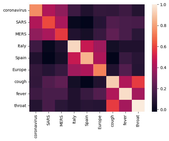
可以看到,嵌入向量成功捕获了不同术语的含义。每个单词都与其所在簇的其他单词相似(即“coronavirus”与“SARS”和“MERS”高度相关),但与其他簇的术语不同(即“SARS”与“Spain”之间的相似度接近于 0)。
现在,我们来看看如何使用这些嵌入向量解决特定任务。
SciCite:引用意图分类
本部分介绍了将嵌入向量用于下游任务(如文本分类)的方法。我们将使用 TensorFlow 数据集中的 SciCite 数据集对学术论文中的引文意图进行分类。给定一个带有学术论文引文的句子,对引文的主要意图进行分类:是背景信息、使用方法,还是比较结果。
builder = tfds.builder(name='scicite')
builder.download_and_prepare()
train_data, validation_data, test_data = builder.as_dataset(
    split=('train', 'validation', 'test'),
    as_supervised=True)
Let's take a look at a few labeled examples from the training set
NUM_EXAMPLES =   10

TEXT_FEATURE_NAME = builder.info.supervised_keys[0]
LABEL_NAME = builder.info.supervised_keys[1]

def label2str(numeric_label):
  m = builder.info.features[LABEL_NAME].names
  return m[numeric_label]

data = next(iter(train_data.batch(NUM_EXAMPLES)))


pd.DataFrame({
    TEXT_FEATURE_NAME: [ex.numpy().decode('utf8') for ex in data[0]],
    LABEL_NAME: [label2str(x) for x in data[1]]
})
训练引用意图分类器
我们将使用 Keras 在 SciCite 数据集上对分类器进行训练。我们构建一个模型,该模型使用 CORD-19 嵌入向量,并在顶部具有一个分类层。
Hyperparameters
EMBEDDING = 'https://tfhub.dev/tensorflow/cord-19/swivel-128d/3'
TRAINABLE_MODULE = False

hub_layer = hub.KerasLayer(EMBEDDING, input_shape=[],
                           dtype=tf.string, trainable=TRAINABLE_MODULE)

model = tf.keras.Sequential()
model.add(hub_layer)
model.add(tf.keras.layers.Dense(3))
model.summary()
model.compile(optimizer='adam',
              loss=tf.keras.losses.SparseCategoricalCrossentropy(from_logits=True),
              metrics=['accuracy'])
WARNING:tensorflow:Please fix your imports. Module tensorflow.python.training.tracking.data_structures has been moved to tensorflow.python.trackable.data_structures. The old module will be deleted in version 2.11.
WARNING:tensorflow:Please fix your imports. Module tensorflow.python.training.tracking.data_structures has been moved to tensorflow.python.trackable.data_structures. The old module will be deleted in version 2.11.
WARNING:tensorflow:From /tmpfs/src/tf_docs_env/lib/python3.9/site-packages/tensorflow/python/autograph/pyct/static_analysis/liveness.py:83: Analyzer.lamba_check (from tensorflow.python.autograph.pyct.static_analysis.liveness) is deprecated and will be removed after 2023-09-23.
Instructions for updating:
Lambda fuctions will be no more assumed to be used in the statement where they are used, or at least in the same block. https://github.com/tensorflow/tensorflow/issues/56089
Model: "sequential"
_________________________________________________________________
 Layer (type)                Output Shape              Param #
=================================================================
 keras_layer (KerasLayer)    (None, 128)               17301632

 dense (Dense)               (None, 3)                 387

=================================================================
Total params: 17,302,019
Trainable params: 387
Non-trainable params: 17,301,632
_________________________________________________________________
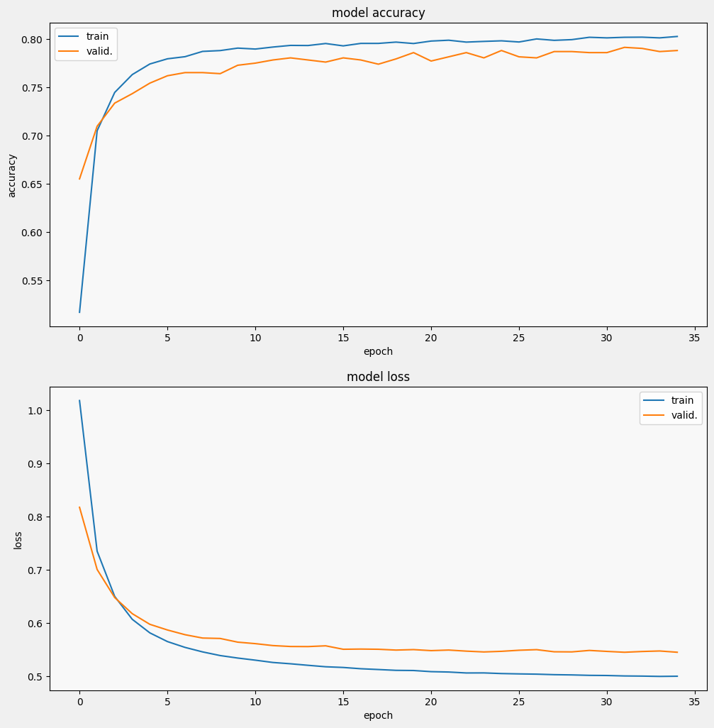
训练并评估模型
让我们训练并评估模型以查看在 SciCite 任务上的性能。
EPOCHS = 35
BATCH_SIZE = 32

history = model.fit(train_data.shuffle(10000).batch(BATCH_SIZE),
                    epochs=EPOCHS,
                    validation_data=validation_data.batch(BATCH_SIZE),
                    verbose=1)
Epoch 1/35
257/257 [==============================] - 3s 5ms/step - loss: 1.0181 - accuracy: 0.5166 - val_loss: 0.8177 - val_accuracy: 0.6550
Epoch 2/35
257/257 [==============================] - 1s 4ms/step - loss: 0.7353 - accuracy: 0.7049 - val_loss: 0.7010 - val_accuracy: 0.7096
Epoch 3/35
257/257 [==============================] - 1s 4ms/step - loss: 0.6503 - accuracy: 0.7447 - val_loss: 0.6482 - val_accuracy: 0.7336
Epoch 4/35
257/257 [==============================] - 2s 4ms/step - loss: 0.6073 - accuracy: 0.7632 - val_loss: 0.6179 - val_accuracy: 0.7434
Epoch 5/35
257/257 [==============================] - 2s 5ms/step - loss: 0.5819 - accuracy: 0.7742 - val_loss: 0.5979 - val_accuracy: 0.7544
Epoch 6/35
257/257 [==============================] - 1s 4ms/step - loss: 0.5655 - accuracy: 0.7796 - val_loss: 0.5873 - val_accuracy: 0.7620
Epoch 7/35
257/257 [==============================] - 1s 4ms/step - loss: 0.5546 - accuracy: 0.7818 - val_loss: 0.5784 - val_accuracy: 0.7653
Epoch 8/35
257/257 [==============================] - 1s 4ms/step - loss: 0.5461 - accuracy: 0.7873 - val_loss: 0.5722 - val_accuracy: 0.7653
Epoch 9/35
257/257 [==============================] - 2s 4ms/step - loss: 0.5393 - accuracy: 0.7881 - val_loss: 0.5714 - val_accuracy: 0.7642
Epoch 10/35
257/257 [==============================] - 1s 4ms/step - loss: 0.5346 - accuracy: 0.7907 - val_loss: 0.5644 - val_accuracy: 0.7729
Epoch 11/35
257/257 [==============================] - 1s 4ms/step - loss: 0.5306 - accuracy: 0.7897 - val_loss: 0.5616 - val_accuracy: 0.7751
Epoch 12/35
257/257 [==============================] - 1s 4ms/step - loss: 0.5263 - accuracy: 0.7918 - val_loss: 0.5580 - val_accuracy: 0.7784
Epoch 13/35
257/257 [==============================] - 1s 4ms/step - loss: 0.5238 - accuracy: 0.7935 - val_loss: 0.5563 - val_accuracy: 0.7806
Epoch 14/35
257/257 [==============================] - 1s 4ms/step - loss: 0.5210 - accuracy: 0.7934 - val_loss: 0.5561 - val_accuracy: 0.7784
Epoch 15/35
257/257 [==============================] - 1s 4ms/step - loss: 0.5182 - accuracy: 0.7955 - val_loss: 0.5576 - val_accuracy: 0.7762
Epoch 16/35
257/257 [==============================] - 1s 4ms/step - loss: 0.5169 - accuracy: 0.7930 - val_loss: 0.5511 - val_accuracy: 0.7806
Epoch 17/35
257/257 [==============================] - 1s 4ms/step - loss: 0.5145 - accuracy: 0.7956 - val_loss: 0.5515 - val_accuracy: 0.7784
Epoch 18/35
257/257 [==============================] - 1s 4ms/step - loss: 0.5130 - accuracy: 0.7956 - val_loss: 0.5511 - val_accuracy: 0.7740
Epoch 19/35
257/257 [==============================] - 1s 4ms/step - loss: 0.5115 - accuracy: 0.7969 - val_loss: 0.5495 - val_accuracy: 0.7795
Epoch 20/35
257/257 [==============================] - 1s 4ms/step - loss: 0.5112 - accuracy: 0.7955 - val_loss: 0.5504 - val_accuracy: 0.7860
Epoch 21/35
257/257 [==============================] - 1s 4ms/step - loss: 0.5090 - accuracy: 0.7980 - val_loss: 0.5485 - val_accuracy: 0.7773
Epoch 22/35
257/257 [==============================] - 1s 4ms/step - loss: 0.5083 - accuracy: 0.7989 - val_loss: 0.5496 - val_accuracy: 0.7817
Epoch 23/35
257/257 [==============================] - 1s 4ms/step - loss: 0.5066 - accuracy: 0.7969 - val_loss: 0.5476 - val_accuracy: 0.7860
Epoch 24/35
257/257 [==============================] - 1s 4ms/step - loss: 0.5067 - accuracy: 0.7977 - val_loss: 0.5461 - val_accuracy: 0.7806
Epoch 25/35
257/257 [==============================] - 1s 4ms/step - loss: 0.5055 - accuracy: 0.7983 - val_loss: 0.5472 - val_accuracy: 0.7882
Epoch 26/35
257/257 [==============================] - 1s 4ms/step - loss: 0.5048 - accuracy: 0.7970 - val_loss: 0.5492 - val_accuracy: 0.7817
Epoch 27/35
257/257 [==============================] - 1s 4ms/step - loss: 0.5043 - accuracy: 0.8002 - val_loss: 0.5504 - val_accuracy: 0.7806
Epoch 28/35
257/257 [==============================] - 1s 4ms/step - loss: 0.5034 - accuracy: 0.7988 - val_loss: 0.5464 - val_accuracy: 0.7871
Epoch 29/35
257/257 [==============================] - 1s 4ms/step - loss: 0.5029 - accuracy: 0.7995 - val_loss: 0.5462 - val_accuracy: 0.7871
Epoch 30/35
257/257 [==============================] - 1s 4ms/step - loss: 0.5021 - accuracy: 0.8019 - val_loss: 0.5489 - val_accuracy: 0.7860
Epoch 31/35
257/257 [==============================] - 1s 4ms/step - loss: 0.5018 - accuracy: 0.8013 - val_loss: 0.5471 - val_accuracy: 0.7860
Epoch 32/35
257/257 [==============================] - 1s 5ms/step - loss: 0.5010 - accuracy: 0.8019 - val_loss: 0.5455 - val_accuracy: 0.7915
Epoch 33/35
257/257 [==============================] - 1s 4ms/step - loss: 0.5007 - accuracy: 0.8021 - val_loss: 0.5469 - val_accuracy: 0.7904
Epoch 34/35
257/257 [==============================] - 1s 4ms/step - loss: 0.5001 - accuracy: 0.8013 - val_loss: 0.5479 - val_accuracy: 0.7871
Epoch 35/35
257/257 [==============================] - 1s 4ms/step - loss: 0.5004 - accuracy: 0.8028 - val_loss: 0.5455 - val_accuracy: 0.7882
from matplotlib import pyplot as plt
def display_training_curves(training, validation, title, subplot):
  if subplot%10==1: # set up the subplots on the first call
    plt.subplots(figsize=(10,10), facecolor='#F0F0F0')
    plt.tight_layout()
  ax = plt.subplot(subplot)
  ax.set_facecolor('#F8F8F8')
  ax.plot(training)
  ax.plot(validation)
  ax.set_title('model '+ title)
  ax.set_ylabel(title)
  ax.set_xlabel('epoch')
  ax.legend(['train', 'valid.'])
display_training_curves(history.history['accuracy'], history.history['val_accuracy'], 'accuracy', 211)
display_training_curves(history.history['loss'], history.history['val_loss'], 'loss', 212)
/tmpfs/tmp/ipykernel_21774/4094752860.py:6: MatplotlibDeprecationWarning: Auto-removal of overlapping axes is deprecated since 3.6 and will be removed two minor releases later; explicitly call ax.remove() as needed.
  ax = plt.subplot(subplot)
评估模型
我们来看看模型的表现。模型将返回两个值:损失(表示错误的数字,值越低越好)和准确率。
results = model.evaluate(test_data.batch(512), verbose=2)

for name, value in zip(model.metrics_names, results):
  print('%s: %.3f' % (name, value))
4/4 - 0s - loss: 0.5379 - accuracy: 0.7848 - 291ms/epoch - 73ms/step
loss: 0.538
accuracy: 0.785
可以看到,损失迅速减小,而准确率迅速提高。我们绘制一些样本来检查预测与真实标签的关系:
prediction_dataset = next(iter(test_data.batch(20)))

prediction_texts = [ex.numpy().decode('utf8') for ex in prediction_dataset[0]]
prediction_labels = [label2str(x) for x in prediction_dataset[1]]

predictions = [
    label2str(x) for x in np.argmax(model.predict(prediction_texts), axis=-1)]


pd.DataFrame({
    TEXT_FEATURE_NAME: prediction_texts,
    LABEL_NAME: prediction_labels,
    'prediction': predictions
})
1/1 [==============================] - 0s 150ms/step
可以看到,对于此随机样本,模型大多数时候都会预测正确的标签,这表明它可以很好地嵌入科学句子。
后续计划
现在,您已经对 TF-Hub 中的 CORD-19 Swivel 嵌入向量有了更多了解,我们鼓励您参加 CORD-19 Kaggle 竞赛,为从 COVID-19 相关学术文本中获得更深入的科学洞见做出贡献。
- 参加 CORD-19 Kaggle Challenge
- 详细了解 COVID-19 开放研究数据集 (CORD-19)
- 访问 https://tfhub.dev/tensorflow/cord-19/swivel-128d/3,参阅文档并详细了解 TF-Hub 嵌入向量
- 使用 TensorFlow Embedding Projector 探索 CORD-19 嵌入向量空间