
| |
|
 在 GitHub 上查看源代码 在 GitHub 上查看源代码
|
|
TF-Hub 是一个平台,用于共享打包为可重用资源的机器学习专业知识,尤其是经过预训练的模块。在本教程中,我们将使用 TF-Hub 文本嵌入向量模块来训练具有合理基线准确率的简单情感分类器。之后,我们会将预测结果提交给 Kaggle。
有关使用 TF-Hub 进行文本分类的更详细教程,以及提高准确率的后续步骤,请查看使用 TF-Hub 进行分本分类。
设置
pip install -q kaggleimport tensorflow as tf
import tensorflow_hub as hub
import matplotlib.pyplot as plt
import numpy as np
import pandas as pd
import seaborn as sns
import zipfile
from sklearn import model_selection
2022-12-14 21:06:07.262712: W tensorflow/compiler/xla/stream_executor/platform/default/dso_loader.cc:64] Could not load dynamic library 'libnvinfer.so.7'; dlerror: libnvinfer.so.7: cannot open shared object file: No such file or directory
2022-12-14 21:06:07.262817: W tensorflow/compiler/xla/stream_executor/platform/default/dso_loader.cc:64] Could not load dynamic library 'libnvinfer_plugin.so.7'; dlerror: libnvinfer_plugin.so.7: cannot open shared object file: No such file or directory
2022-12-14 21:06:07.262829: W tensorflow/compiler/tf2tensorrt/utils/py_utils.cc:38] TF-TRT Warning: Cannot dlopen some TensorRT libraries. If you would like to use Nvidia GPU with TensorRT, please make sure the missing libraries mentioned above are installed properly.
由于本教程将使用 Kaggle 中的数据集,因此需要为您的 Kaggle 帐号创建 API 令牌,并将其上传到 Colab 环境。
import os
import pathlib

# Upload the API token.
def get_kaggle():
  try:
    import kaggle
    return kaggle
  except OSError:
    pass

  token_file = pathlib.Path("~/.kaggle/kaggle.json").expanduser()
  token_file.parent.mkdir(exist_ok=True, parents=True)

  try:
    from google.colab import files
  except ImportError:
    raise ValueError("Could not find kaggle token.")

  uploaded = files.upload()
  token_content = uploaded.get('kaggle.json', None)
  if token_content:
    token_file.write_bytes(token_content)
    token_file.chmod(0o600)
  else:
    raise ValueError('Need a file named "kaggle.json"')

  import kaggle
  return kaggle


kaggle = get_kaggle()
开始
数据
我们将尝试完成 Kaggle 的 Sentiment Analysis on Movie Reviews 任务。数据集由 Rotten Tomatoes 电影评论中符合句法的子短语组成。任务是采用五分制将短语标记为负面或正面。
在使用此 API 下载数据之前,您必须接受竞赛规则。
SENTIMENT_LABELS = [
    "negative", "somewhat negative", "neutral", "somewhat positive", "positive"
]

# Add a column with readable values representing the sentiment.
def add_readable_labels_column(df, sentiment_value_column):
  df["SentimentLabel"] = df[sentiment_value_column].replace(
      range(5), SENTIMENT_LABELS)

# Download data from Kaggle and create a DataFrame.
def load_data_from_zip(path):
  with zipfile.ZipFile(path, "r") as zip_ref:
    name = zip_ref.namelist()[0]
    with zip_ref.open(name) as zf:
      return pd.read_csv(zf, sep="\t", index_col=0)


# The data does not come with a validation set so we'll create one from the
# training set.
def get_data(competition, train_file, test_file, validation_set_ratio=0.1):
  data_path = pathlib.Path("data")
  kaggle.api.competition_download_files(competition, data_path)
  competition_path = (data_path/competition)
  competition_path.mkdir(exist_ok=True, parents=True)
  competition_zip_path = competition_path.with_suffix(".zip")

  with zipfile.ZipFile(competition_zip_path, "r") as zip_ref:
    zip_ref.extractall(competition_path)

  train_df = load_data_from_zip(competition_path/train_file)
  test_df = load_data_from_zip(competition_path/test_file)

  # Add a human readable label.
  add_readable_labels_column(train_df, "Sentiment")

  # We split by sentence ids, because we don't want to have phrases belonging
  # to the same sentence in both training and validation set.
  train_indices, validation_indices = model_selection.train_test_split(
      np.unique(train_df["SentenceId"]),
      test_size=validation_set_ratio,
      random_state=0)

  validation_df = train_df[train_df["SentenceId"].isin(validation_indices)]
  train_df = train_df[train_df["SentenceId"].isin(train_indices)]
  print("Split the training data into %d training and %d validation examples." %
        (len(train_df), len(validation_df)))

  return train_df, validation_df, test_df


train_df, validation_df, test_df = get_data(
    "sentiment-analysis-on-movie-reviews",
    "train.tsv.zip", "test.tsv.zip")
Split the training data into 140315 training and 15745 validation examples.
注:本竞赛的任务不是对整个评论进行评分,而是对评论中的各个短语进行评分。这是一项更加艰巨的任务。
train_df.head(20)
训练模型
注:我们也可以将此任务建模为回归模型,请参阅使用 TF-Hub 进行文本分类。
class MyModel(tf.keras.Model):
  def __init__(self, hub_url):
    super().__init__()
    self.hub_url = hub_url
    self.embed = hub.load(self.hub_url).signatures['default']
    self.sequential = tf.keras.Sequential([
      tf.keras.layers.Dense(500),
      tf.keras.layers.Dense(100),
      tf.keras.layers.Dense(5),
    ])

  def call(self, inputs):
    phrases = inputs['Phrase'][:,0]
    embedding = 5*self.embed(phrases)['default']
    return self.sequential(embedding)

  def get_config(self):
    return {"hub_url":self.hub_url}
model = MyModel("https://tfhub.dev/google/nnlm-en-dim128/1")
model.compile(
    loss = tf.losses.SparseCategoricalCrossentropy(from_logits=True),
    optimizer=tf.optimizers.Adam(),
    metrics = [tf.keras.metrics.SparseCategoricalAccuracy(name="accuracy")])
history = model.fit(x=dict(train_df), y=train_df['Sentiment'],
          validation_data=(dict(validation_df), validation_df['Sentiment']),
          epochs = 25)
Epoch 1/25
4385/4385 [==============================] - 14s 3ms/step - loss: 1.0246 - accuracy: 0.5858 - val_loss: 0.9966 - val_accuracy: 0.5968
Epoch 2/25
4385/4385 [==============================] - 12s 3ms/step - loss: 0.9997 - accuracy: 0.5953 - val_loss: 0.9854 - val_accuracy: 0.5933
Epoch 3/25
4385/4385 [==============================] - 12s 3ms/step - loss: 0.9951 - accuracy: 0.5971 - val_loss: 0.9866 - val_accuracy: 0.5996
Epoch 4/25
4385/4385 [==============================] - 12s 3ms/step - loss: 0.9930 - accuracy: 0.5980 - val_loss: 0.9843 - val_accuracy: 0.5943
Epoch 5/25
4385/4385 [==============================] - 13s 3ms/step - loss: 0.9919 - accuracy: 0.5971 - val_loss: 0.9815 - val_accuracy: 0.5980
Epoch 6/25
4385/4385 [==============================] - 12s 3ms/step - loss: 0.9903 - accuracy: 0.5977 - val_loss: 0.9844 - val_accuracy: 0.5921
Epoch 7/25
4385/4385 [==============================] - 12s 3ms/step - loss: 0.9892 - accuracy: 0.5984 - val_loss: 0.9821 - val_accuracy: 0.5952
Epoch 8/25
4385/4385 [==============================] - 12s 3ms/step - loss: 0.9889 - accuracy: 0.5975 - val_loss: 0.9838 - val_accuracy: 0.5881
Epoch 9/25
4385/4385 [==============================] - 13s 3ms/step - loss: 0.9885 - accuracy: 0.5985 - val_loss: 0.9816 - val_accuracy: 0.5921
Epoch 10/25
4385/4385 [==============================] - 13s 3ms/step - loss: 0.9879 - accuracy: 0.5986 - val_loss: 0.9821 - val_accuracy: 0.5964
Epoch 11/25
4385/4385 [==============================] - 13s 3ms/step - loss: 0.9876 - accuracy: 0.5998 - val_loss: 0.9804 - val_accuracy: 0.5945
Epoch 12/25
4385/4385 [==============================] - 13s 3ms/step - loss: 0.9876 - accuracy: 0.5991 - val_loss: 0.9837 - val_accuracy: 0.5915
Epoch 13/25
4385/4385 [==============================] - 12s 3ms/step - loss: 0.9875 - accuracy: 0.5994 - val_loss: 0.9790 - val_accuracy: 0.5953
Epoch 14/25
4385/4385 [==============================] - 12s 3ms/step - loss: 0.9871 - accuracy: 0.5990 - val_loss: 0.9855 - val_accuracy: 0.5985
Epoch 15/25
4385/4385 [==============================] - 12s 3ms/step - loss: 0.9868 - accuracy: 0.5989 - val_loss: 0.9804 - val_accuracy: 0.5952
Epoch 16/25
4385/4385 [==============================] - 13s 3ms/step - loss: 0.9871 - accuracy: 0.5995 - val_loss: 0.9797 - val_accuracy: 0.5940
Epoch 17/25
4385/4385 [==============================] - 13s 3ms/step - loss: 0.9866 - accuracy: 0.5994 - val_loss: 0.9787 - val_accuracy: 0.5955
Epoch 18/25
4385/4385 [==============================] - 13s 3ms/step - loss: 0.9866 - accuracy: 0.5996 - val_loss: 0.9794 - val_accuracy: 0.5971
Epoch 19/25
4385/4385 [==============================] - 13s 3ms/step - loss: 0.9864 - accuracy: 0.5998 - val_loss: 0.9734 - val_accuracy: 0.5975
Epoch 20/25
4385/4385 [==============================] - 12s 3ms/step - loss: 0.9862 - accuracy: 0.5990 - val_loss: 0.9796 - val_accuracy: 0.5954
Epoch 21/25
4385/4385 [==============================] - 12s 3ms/step - loss: 0.9864 - accuracy: 0.5991 - val_loss: 0.9755 - val_accuracy: 0.6002
Epoch 22/25
4385/4385 [==============================] - 12s 3ms/step - loss: 0.9862 - accuracy: 0.5997 - val_loss: 0.9811 - val_accuracy: 0.5983
Epoch 23/25
4385/4385 [==============================] - 13s 3ms/step - loss: 0.9860 - accuracy: 0.5999 - val_loss: 0.9815 - val_accuracy: 0.5903
Epoch 24/25
4385/4385 [==============================] - 12s 3ms/step - loss: 0.9862 - accuracy: 0.6004 - val_loss: 0.9816 - val_accuracy: 0.5918
Epoch 25/25
4385/4385 [==============================] - 13s 3ms/step - loss: 0.9860 - accuracy: 0.5993 - val_loss: 0.9786 - val_accuracy: 0.5959
预测
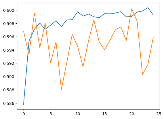
为验证集和训练集运行预测。
plt.plot(history.history['accuracy'])
plt.plot(history.history['val_accuracy'])
[<matplotlib.lines.Line2D at 0x7f550c6f09a0>]
train_eval_result = model.evaluate(dict(train_df), train_df['Sentiment'])
validation_eval_result = model.evaluate(dict(validation_df), validation_df['Sentiment'])

print(f"Training set accuracy: {train_eval_result[1]}")
print(f"Validation set accuracy: {validation_eval_result[1]}")
4385/4385 [==============================] - 12s 3ms/step - loss: 0.9820 - accuracy: 0.6014
493/493 [==============================] - 1s 2ms/step - loss: 0.9786 - accuracy: 0.5959
Training set accuracy: 0.6014040112495422
Validation set accuracy: 0.5959352254867554
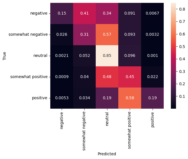
混淆矩阵
另一个非常有趣的统计数据(尤其对于多类问题而言)是混淆矩阵。混淆矩阵允许可视化显示正确和错误标记的样本的比例。我们可以很容易看出分类器出现了多大偏差,以及标签分布是否有意义。理想情况下,预测中的最大数值应沿对角线分布。
predictions = model.predict(dict(validation_df))
predictions = tf.argmax(predictions, axis=-1)
predictions
493/493 [==============================] - 1s 2ms/step
<tf.Tensor: shape=(15745,), dtype=int64, numpy=array([2, 2, 2, ..., 2, 2, 2])>
cm = tf.math.confusion_matrix(validation_df['Sentiment'], predictions)
cm = cm/cm.numpy().sum(axis=1)[:, tf.newaxis]
sns.heatmap(
    cm, annot=True,
    xticklabels=SENTIMENT_LABELS,
    yticklabels=SENTIMENT_LABELS)
plt.xlabel("Predicted")
plt.ylabel("True")
Text(50.72222222222221, 0.5, 'True')
我们可以将以下代码粘贴到代码单元,然后执行该代码,从而轻松将预测值提交回 Kaggle:
test_predictions = model.predict(dict(test_df))
test_predictions = np.argmax(test_predictions, axis=-1)

result_df = test_df.copy()

result_df["Predictions"] = test_predictions

result_df.to_csv(
    "predictions.csv",
    columns=["Predictions"],
    header=["Sentiment"])
kaggle.api.competition_submit("predictions.csv", "Submitted from Colab",
                              "sentiment-analysis-on-movie-reviews")
提交后,查看排行榜了解您的表现。