MIT লাইসেন্সের অধীনে লাইসেন্সপ্রাপ্ত
# Permission is hereby granted, free of charge, to any person obtaining a copy
# of this software and associated documentation files (the "Software"), to deal
# in the Software without restriction, including without limitation the rights
# to use, copy, modify, merge, publish, distribute, sublicense, and/or sell
# copies of the Software, and to permit persons to whom the Software is
# furnished to do so, subject to the following conditions:
#
# The above copyright notice and this permission notice shall be included in all
# copies or substantial portions of the Software.
#
# THE SOFTWARE IS PROVIDED "AS IS", WITHOUT WARRANTY OF ANY KIND, EXPRESS OR
# IMPLIED, INCLUDING BUT NOT LIMITED TO THE WARRANTIES OF MERCHANTABILITY,
# FITNESS FOR A PARTICULAR PURPOSE AND NONINFRINGEMENT. IN NO EVENT SHALL THE
# AUTHORS OR COPYRIGHT HOLDERS BE LIABLE FOR ANY CLAIM, DAMAGES OR OTHER
# LIABILITY, WHETHER IN AN ACTION OF CONTRACT, TORT OR OTHERWISE, ARISING FROM,
# OUT OF OR IN CONNECTION WITH THE SOFTWARE OR THE USE OR OTHER DEALINGS IN THE
# SOFTWARE.
| | |  GitHub-এ উৎস দেখুন GitHub-এ উৎস দেখুন | |
2020 সালের গোড়ার দিকে COVID-19-এর বিস্তারকে ধীর করার জন্য, ইউরোপীয় দেশগুলি অ-ফার্মাসিউটিক্যাল হস্তক্ষেপগুলি গ্রহণ করেছে যেমন অ-প্রয়োজনীয় ব্যবসা বন্ধ করা, ব্যক্তিগত ক্ষেত্রে বিচ্ছিন্ন করা, ভ্রমণ নিষেধাজ্ঞা এবং সামাজিক দূরত্বকে উত্সাহিত করার জন্য অন্যান্য ব্যবস্থা। ইম্পেরিয়াল কলেজ COVID -19 রেসপন্স টিম তাদের কাগজে এই মাত্রাগুলির কার্যকারিতা বিশ্লেষণ "সংক্রমণ সংখ্যা এবং 11 ইউরোপীয় দেশগুলিতে COVID -19 নন-ফার্মাসিউটিক্যাল হস্তক্ষেপ প্রভাব দেখায়" , একটি মেকানিজম সঙ্গে মিলিত একটি Bayesian হায়ারারকিকাল মডেল ব্যবহার মহামারী সংক্রান্ত মডেল।
এই Colab-এ সেই বিশ্লেষণের একটি TensorFlow সম্ভাব্যতা (TFP) প্রয়োগ রয়েছে, যা নিম্নরূপ সংগঠিত:
- "মডেল সেটআপ" রোগের সংক্রমণ এবং এর ফলে মৃত্যুর জন্য মহামারী সংক্রান্ত মডেলকে সংজ্ঞায়িত করে, মডেল প্যারামিটারের উপর বায়েসিয়ান পূর্বের বন্টন এবং প্যারামিটার মানগুলির উপর শর্তসাপেক্ষে মৃত্যুর সংখ্যা বন্টন।
- "ডেটা প্রিপ্রসেসিং" প্রতিটি দেশে হস্তক্ষেপের সময় এবং ধরণ, সময়ের সাথে সাথে মৃত্যুর সংখ্যা এবং সংক্রামিতদের জন্য আনুমানিক মৃত্যুর হারের উপর ডেটা লোড করে।
- "মডেল ইনফরেন্স" একটি বায়েসিয়ান হায়ারার্কিক্যাল মডেল তৈরি করে এবং প্যারামিটারের উপর পশ্চাৎভাগের বন্টন থেকে নমুনা নিতে হ্যামিলটোনিয়ান মন্টে কার্লো (HMC) চালায়।
- "ফলাফল" হস্তক্ষেপের অনুপস্থিতিতে পূর্বাভাসিত মৃত্যু, এবং কাউন্টারফ্যাকচুয়াল মৃত্যুর মতো আগ্রহের পরিমাণের জন্য পরবর্তী ভবিষ্যদ্বাণীমূলক বিতরণ দেখায়।
কাগজ প্রমাণ দেশ প্রতিটি আক্রান্ত ব্যক্তির (দ্বারা প্রেরিত নতুন সংক্রমণ সংখ্যা কমাতে পরিচালিত গেছে\(R_t\)), কিন্তু যে বিশ্বাসযোগ্য অন্তর অন্তর্ভুক্ত \(R_t=1\) (মান যার উপরে মহামারী বিস্তার অব্যাহত) এবং অকাল ছিল হস্তক্ষেপের কার্যকারিতা সম্পর্কে দৃঢ় সিদ্ধান্তে আঁকতে। পত্রিকাটির জন্য স্ট্যান কোড লেখকদের হয় গিটহাব সংগ্রহস্থলের, এবং এই Colab প্রজনন সংস্করণ 2 ।
pip3 install -q git+git://github.com/arviz-devs/arviz.gitpip3 install -q tf-nightly tfp-nightly
আমদানি
import collections
from pprint import pprint

import numpy as np
import pandas as pd

import matplotlib.pyplot as plt

%config InlineBackend.figure_format = 'retina'

import tensorflow.compat.v2 as tf
import tensorflow_probability as tfp
from tensorflow_probability.python.internal import prefer_static as ps

tf.enable_v2_behavior()

# Globally Enable XLA.
# tf.config.optimizer.set_jit(True)

try:
  physical_devices = tf.config.list_physical_devices('GPU')
  tf.config.experimental.set_memory_growth(physical_devices[0], True)
except:
  # Invalid device or cannot modify virtual devices once initialized.
  pass

tfb = tfp.bijectors
tfd = tfp.distributions

DTYPE = np.float32
1 মডেল সেটআপ
1.1 সংক্রমণ এবং মৃত্যুর জন্য যান্ত্রিক মডেল
সংক্রমণ মডেল সময়ের সাথে প্রতিটি দেশে সংক্রমণের সংখ্যা অনুকরণ করে। ইনপুট ডেটা হস্তক্ষেপের সময় এবং ধরন, জনসংখ্যার আকার এবং প্রাথমিক ক্ষেত্রে। প্যারামিটারগুলি হস্তক্ষেপের কার্যকারিতা এবং রোগ সংক্রমণের হার নিয়ন্ত্রণ করে। মৃত্যুর প্রত্যাশিত সংখ্যার মডেলটি পূর্বাভাসিত সংক্রমণের জন্য একটি মৃত্যুর হার প্রয়োগ করে।
সংক্রমণ মডেলটি সিরিয়াল ব্যবধান বন্টন (সংক্রমিত হওয়া এবং অন্য কাউকে সংক্রামিত করার মধ্যে দিনের সংখ্যার মধ্যে বিতরণ) এর সাথে পূর্ববর্তী দৈনিক সংক্রমণের একটি পরিবর্তন করে। প্রতিটি সময় ধাপ অনুযায়ী, সময়ে নতুন সংক্রমণ সংখ্যা \(t\), \(n_t\), হিসাবে গণনা করা হয়
\begin{equation} \sum_{i=0}^{t-1} n_i \mu_t \text{p} (\text{কেউ সংক্রমিত থেকে ধরা } i | \text{নতুন সংক্রমিত at } t) \end{ সমীকরণ} যেখানে \(\mu_t=R_t\) এবং শর্তাধীন সম্ভাব্যতা মধ্যে সংরক্ষিত হয় conv_serial_interval , নিম্নে বর্ণিত।
প্রত্যাশিত মৃত্যুর মডেলটি প্রতিদিনের সংক্রমণ এবং সংক্রমণ এবং মৃত্যুর মধ্যে দিনগুলি বণ্টন করে। অর্থাৎ দিনে প্রত্যাশিত মৃত্যু হয় \(t\) হিসাবে গণনা করা হয়
\ শুরু {সমীকরণ} \ sum_ {i = 0} ^ {টি-1} n_i \ টেক্সট {P (দিনে মৃত্যু \(t\)| দিনে সংক্রমণ \(i\))} \ শেষ {সমীকরণ} যেখানে শর্তসাপেক্ষ সম্ভাব্যতা সংরক্ষিত হয় মধ্যে conv_fatality_rate , নিম্নে বর্ণিত।
from tensorflow_probability.python.internal import broadcast_util as bu

def predict_infections(
    intervention_indicators, population, initial_cases, mu, alpha_hier,
    conv_serial_interval, initial_days, total_days):
  """Predict the number of infections by forward-simulation.

  Args:
    intervention_indicators: Binary array of shape
      `[num_countries, total_days, num_interventions]`, in which `1` indicates
      the intervention is active in that country at that time and `0` indicates
      otherwise.
    population: Vector of length `num_countries`. Population of each country.
    initial_cases: Array of shape `[batch_size, num_countries]`. Number of cases
      in each country at the start of the simulation.
    mu: Array of shape `[batch_size, num_countries]`. Initial reproduction rate
      (R_0) by country.
    alpha_hier: Array of shape `[batch_size, num_interventions]` representing
      the effectiveness of interventions.
    conv_serial_interval: Array of shape
      `[total_days - initial_days, total_days]` output from
      `make_conv_serial_interval`. Convolution kernel for serial interval
      distribution.
    initial_days: Integer, number of sequential days to seed infections after
      the 10th death in a country. (N0 in the authors' Stan code.)
    total_days: Integer, number of days of observed data plus days to forecast.
      (N2 in the authors' Stan code.)
  Returns:
    predicted_infections: Array of shape
      `[total_days, batch_size, num_countries]`. (Batched) predicted number of
      infections over time and by country.
  """
  alpha = alpha_hier - tf.cast(np.log(1.05) / 6.0, DTYPE)

  # Multiply the effectiveness of each intervention in each country (alpha)
  # by the indicator variable for whether the intervention was active and sum
  # over interventions, yielding an array of shape
  # [total_days, batch_size, num_countries] that represents the total effectiveness of
  # all interventions in each country on each day (for a batch of data).
  linear_prediction = tf.einsum(
      'ijk,...k->j...i', intervention_indicators, alpha)

  # Adjust the reproduction rate per country downward, according to the
  # effectiveness of the interventions.
  rt = mu * tf.exp(-linear_prediction, name='reproduction_rate')

  # Initialize storage array for daily infections and seed it with initial
  # cases.
  daily_infections = tf.TensorArray(
      dtype=DTYPE, size=total_days, element_shape=initial_cases.shape)
  for i in range(initial_days):
    daily_infections = daily_infections.write(i, initial_cases)

  # Initialize cumulative cases.
  init_cumulative_infections = initial_cases * initial_days

  # Simulate forward for total_days days.
  cond = lambda i, *_: i < total_days
  def body(i, prev_daily_infections, prev_cumulative_infections):
    # The probability distribution over days j that someone infected on day i
    # caught the virus from someone infected on day j.
    p_infected_on_day = tf.gather(
        conv_serial_interval, i - initial_days, axis=0)

    # Multiply p_infected_on_day by the number previous infections each day and
    # by mu, and sum to obtain new infections on day i. Mu is adjusted by
    # the fraction of the population already infected, so that the population
    # size is the upper limit on the number of infections.
    prev_daily_infections_array = prev_daily_infections.stack()
    to_sum = prev_daily_infections_array * bu.left_justified_expand_dims_like(
        p_infected_on_day, prev_daily_infections_array)
    convolution = tf.reduce_sum(to_sum, axis=0)
    rt_adj = (
        (population - prev_cumulative_infections) / population
        ) * tf.gather(rt, i)
    new_infections = rt_adj * convolution

    # Update the prediction array and the cumulative number of infections.
    daily_infections = prev_daily_infections.write(i, new_infections)
    cumulative_infections = prev_cumulative_infections + new_infections
    return i + 1, daily_infections, cumulative_infections

  _, daily_infections_final, last_cumm_sum = tf.while_loop(
      cond, body,
      (initial_days, daily_infections, init_cumulative_infections),
      maximum_iterations=(total_days - initial_days))
  return daily_infections_final.stack()

def predict_deaths(predicted_infections, ifr_noise, conv_fatality_rate):
  """Expected number of reported deaths by country, by day.

  Args:
    predicted_infections: Array of shape
      `[total_days, batch_size, num_countries]` output from
      `predict_infections`.
    ifr_noise: Array of shape `[batch_size, num_countries]`. Noise in Infection
      Fatality Rate (IFR).
    conv_fatality_rate: Array of shape
      `[total_days - 1, total_days, num_countries]`. Convolutional kernel for
      calculating fatalities, output from `make_conv_fatality_rate`.
  Returns:
    predicted_deaths: Array of shape `[total_days, batch_size, num_countries]`.
      (Batched) predicted number of deaths over time and by country.
  """
  # Multiply the number of infections on day j by the probability of death
  # on day i given infection on day j, and sum over j. This yields the expected
  result_remainder = tf.einsum(
      'i...j,kij->k...j', predicted_infections, conv_fatality_rate) * ifr_noise

  # Concatenate the result with a vector of zeros so that the first day is
  # included.
  result_temp = 1e-15 * predicted_infections[:1]
  return tf.concat([result_temp, result_remainder], axis=0)
1.2 প্রার ওভার প্যারামিটার মান
এখানে আমরা মডেল পরামিতিগুলির উপর যৌথ পূর্ব বন্টন সংজ্ঞায়িত করি। অনেক প্যারামিটার মানকে স্বাধীন বলে ধরে নেওয়া হয়, যেমন পূর্বকে এভাবে প্রকাশ করা যেতে পারে:
\(\text p(\tau, y, \psi, \kappa, \mu, \alpha) = \text p(\tau)\text p(y|\tau)\text p(\psi)\text p(\kappa)\text p(\mu|\kappa)\text p(\alpha)\text p(\epsilon)\)
যা:
- \(\tau\) প্রতি দেশ, প্রাথমিক মামলার সংখ্যা বেশি সূচকীয় বণ্টনের ভাগ হার প্যারামিটার \(y = y_1, ... y_{\text{num_countries} }\)।
- \(\psi\) মৃত্যুর সংখ্যার জন্য ঋণাত্মক দ্বিপদ বিন্যাসের একটি প্যারামিটার।
- \(\kappa\) প্রতিটি দেশের, প্রারম্ভিক প্রজনন সংখ্যা বেশি HalfNormal বিতরণের ভাগ স্কেল প্যারামিটার \(\mu = \mu_1, ..., \mu_{\text{num_countries} }\) (প্রতিটি আক্রান্ত ব্যক্তির দ্বারা প্রেরিত অতিরিক্ত মামলার সংখ্যা ইঙ্গিত)।
- \(\alpha = \alpha_1, ..., \alpha_6\) ছয় হস্তক্ষেপ প্রতিটি কার্যকারিতা নেই।
- \(\epsilon\) (যাকে বলা হয়
ifr_noiseকোডে, লেখক 'স্ট্যান কোড পর) সংক্রমণের নশ্বরতা হার (IFR) এ গোলমাল হয়।
আমরা এই মডেলটিকে একটি TFP জয়েন্ট ডিস্ট্রিবিউশন হিসাবে প্রকাশ করি, TFP বিতরণের একটি প্রকার যা সম্ভাব্য গ্রাফিকাল মডেলগুলির অভিব্যক্তিকে সক্ষম করে।
def make_jd_prior(num_countries, num_interventions):
  return tfd.JointDistributionSequentialAutoBatched([
      # Rate parameter for the distribution of initial cases (tau).
      tfd.Exponential(rate=tf.cast(0.03, DTYPE)),

      # Initial cases for each country.
      lambda tau: tfd.Sample(
          tfd.Exponential(rate=tf.cast(1, DTYPE) / tau),
          sample_shape=num_countries),

      # Parameter in Negative Binomial model for deaths (psi).
      tfd.HalfNormal(scale=tf.cast(5, DTYPE)),

      # Parameter in the distribution over the initial reproduction number, R_0
      # (kappa).
      tfd.HalfNormal(scale=tf.cast(0.5, DTYPE)),

      # Initial reproduction number, R_0, for each country (mu).
      lambda kappa: tfd.Sample(
          tfd.TruncatedNormal(loc=3.28, scale=kappa, low=1e-5, high=1e5),
          sample_shape=num_countries),

      # Impact of interventions (alpha; shared for all countries).
      tfd.Sample(
          tfd.Gamma(tf.cast(0.1667, DTYPE), 1), sample_shape=num_interventions),

      # Multiplicative noise in Infection Fatality Rate.
      tfd.Sample(
          tfd.TruncatedNormal(
              loc=tf.cast(1., DTYPE), scale=0.1, low=1e-5, high=1e5),
              sample_shape=num_countries)
  ])
1.3 পরামিতি মানগুলির শর্তসাপেক্ষে পর্যবেক্ষিত মৃত্যুর সম্ভাবনা
সম্ভাবনা মডেল প্রকাশ \(p(\text{deaths} | \tau, y, \psi, \kappa, \mu, \alpha, \epsilon)\)। এটি প্যারামিটারের উপর শর্তসাপেক্ষে সংক্রমণ এবং প্রত্যাশিত মৃত্যুর সংখ্যার মডেলগুলি প্রয়োগ করে এবং প্রকৃত মৃত্যু একটি নেতিবাচক দ্বিপদ বন্টন অনুসরণ করে অনুমান করে।
def make_likelihood_fn(
    intervention_indicators, population, deaths,
    infection_fatality_rate, initial_days, total_days):

  # Create a mask for the initial days of simulated data, as they are not
  # counted in the likelihood.
  observed_deaths = tf.constant(deaths.T[np.newaxis, ...], dtype=DTYPE)
  mask_temp = deaths != -1
  mask_temp[:, :START_DAYS] = False
  observed_deaths_mask = tf.constant(mask_temp.T[np.newaxis, ...])

  conv_serial_interval = make_conv_serial_interval(initial_days, total_days)
  conv_fatality_rate = make_conv_fatality_rate(
      infection_fatality_rate, total_days)

  def likelihood_fn(tau, initial_cases, psi, kappa, mu, alpha_hier, ifr_noise):
    # Run models for infections and expected deaths
    predicted_infections = predict_infections(
        intervention_indicators, population, initial_cases, mu, alpha_hier,
        conv_serial_interval, initial_days, total_days)
    e_deaths_all_countries = predict_deaths(
        predicted_infections, ifr_noise, conv_fatality_rate)

    # Construct the Negative Binomial distribution for deaths by country.
    mu_m = tf.transpose(e_deaths_all_countries, [1, 0, 2])
    psi_m = psi[..., tf.newaxis, tf.newaxis]
    probs = tf.clip_by_value(mu_m / (mu_m + psi_m), 1e-9, 1.)
    likelihood_elementwise = tfd.NegativeBinomial(
        total_count=psi_m, probs=probs).log_prob(observed_deaths)
    return tf.reduce_sum(
        tf.where(observed_deaths_mask,
                likelihood_elementwise,
                tf.zeros_like(likelihood_elementwise)),
        axis=[-2, -1])

  return likelihood_fn
1.4 সংক্রমণের কারণে মৃত্যুর সম্ভাবনা
এই বিভাগটি সংক্রমণের পরের দিনগুলিতে মৃত্যুর বিতরণ গণনা করে। এটি অনুমান করে যে সংক্রমণ থেকে মৃত্যু পর্যন্ত সময় দুটি গামা-ভেরিয়েট পরিমাণের সমষ্টি, যা সংক্রমণ থেকে রোগের সূত্রপাত এবং শুরু থেকে মৃত্যুর সময়কে প্রতিনিধিত্ব করে। সময়-টু-মৃত্যুর বন্টন থেকে সংক্রমণ মৃত্যুর হার ডেটা সঙ্গে মিলিত হয় verity এট অল। (2020) সংক্রমণ নিম্নলিখিত দিনে মৃত্যুর সম্ভাবনা গনা।
def daily_fatality_probability(infection_fatality_rate, total_days):
  """Computes the probability of death `d` days after infection."""

  # Convert from alternative Gamma parametrization and construct distributions
  # for number of days from infection to onset and onset to death.
  concentration1 = tf.cast((1. / 0.86)**2, DTYPE)
  rate1 = concentration1 / 5.1
  concentration2 = tf.cast((1. / 0.45)**2, DTYPE)
  rate2 = concentration2 / 18.8
  infection_to_onset = tfd.Gamma(concentration=concentration1, rate=rate1)
  onset_to_death = tfd.Gamma(concentration=concentration2, rate=rate2)

  # Create empirical distribution for number of days from infection to death.
  inf_to_death_dist = tfd.Empirical(
      infection_to_onset.sample([5e6]) + onset_to_death.sample([5e6]))

  # Subtract the CDF value at day i from the value at day i + 1 to compute the
  # probability of death on day i given infection on day 0, and given that
  # death (not recovery) is the outcome.
  times = np.arange(total_days + 1., dtype=DTYPE) + 0.5
  cdf = inf_to_death_dist.cdf(times).numpy()
  f_before_ifr = cdf[1:] - cdf[:-1]
  # Explicitly set the zeroth value to the empirical cdf at time 1.5, to include
  # the mass between time 0 and time .5.
  f_before_ifr[0] = cdf[1]

  # Multiply the daily fatality rates conditional on infection and eventual
  # death (f_before_ifr) by the infection fatality rates (probability of death
  # given intection) to obtain the probability of death on day i conditional
  # on infection on day 0.
  return infection_fatality_rate[..., np.newaxis] * f_before_ifr

def make_conv_fatality_rate(infection_fatality_rate, total_days):
  """Computes the probability of death on day `i` given infection on day `j`."""
  p_fatal_all_countries = daily_fatality_probability(
      infection_fatality_rate, total_days)

  # Use the probability of death d days after infection in each country
  # to build an array of shape [total_days - 1, total_days, num_countries],
  # where the element [i, j, c] is the probability of death on day i+1 given
  # infection on day j in country c.
  conv_fatality_rate = np.zeros(
      [total_days - 1, total_days, p_fatal_all_countries.shape[0]])
  for n in range(1, total_days):
    conv_fatality_rate[n - 1, 0:n, :] = (
        p_fatal_all_countries[:, n - 1::-1]).T
  return tf.constant(conv_fatality_rate, dtype=DTYPE)
1.5 সিরিয়াল ব্যবধান
ক্রমিক ব্যবধান হল রোগ সংক্রমণের একটি শৃঙ্খলে ক্রমাগত মামলার মধ্যে সময়, এবং এটি গামা বিতরণ বলে ধরে নেওয়া হয়। আমরা সিরিয়াল ব্যবধান বন্টন ব্যবহার সম্ভাব্যতা সেদিন সংক্রমিত একজন ব্যক্তি গনা \(i\) পূর্বে দিনে সংক্রমিত একজন ব্যক্তি থেকে ভাইরাস ধরা \(j\) ( conv_serial_interval আর্গুমেন্ট প্রাপ্ত করতে predict_infections )।
def make_conv_serial_interval(initial_days, total_days):
  """Construct the convolutional kernel for infection timing."""

  g = tfd.Gamma(tf.cast(1. / (0.62**2), DTYPE), 1./(6.5*0.62**2))
  g_cdf = g.cdf(np.arange(total_days, dtype=DTYPE))

  # Approximate the probability mass function for the number of days between
  # successive infections.
  serial_interval = g_cdf[1:] - g_cdf[:-1]

  # `conv_serial_interval` is an array of shape
  # [total_days - initial_days, total_days] in which entry [i, j] contains the
  # probability that an individual infected on day i + initial_days caught the
  # virus from someone infected on day j.
  conv_serial_interval = np.zeros([total_days - initial_days, total_days])
  for n in range(initial_days, total_days):
    conv_serial_interval[n - initial_days, 0:n] = serial_interval[n - 1::-1]
  return tf.constant(conv_serial_interval, dtype=DTYPE)
2 ডেটা প্রিপ্রসেসিং
COUNTRIES = [
    'Austria',
    'Belgium',
    'Denmark',
    'France',
    'Germany',
    'Italy',
    'Norway',
    'Spain',
    'Sweden',
    'Switzerland',
    'United_Kingdom'
]
2.1 হস্তক্ষেপ ডেটা আনুন এবং প্রিপ্রসেস করুন৷
raw_interventions = pd.read_csv(
    'https://raw.githubusercontent.com/ImperialCollegeLondon/covid19model/master/data/interventions.csv')

raw_interventions['Date effective'] = pd.to_datetime(
    raw_interventions['Date effective'], dayfirst=True)
interventions = raw_interventions.pivot(index='Country', columns='Type', values='Date effective')

# If any interventions happened after the lockdown, use the date of the lockdown.
for col in interventions.columns:
  idx = interventions[col] > interventions['Lockdown']
  interventions.loc[idx, col] = interventions[idx]['Lockdown']

num_countries = len(COUNTRIES)
2.2 কেস/মৃত্যুর ডেটা আনুন এবং হস্তক্ষেপে যোগ দিন
# Load the case data
data = pd.read_csv('https://raw.githubusercontent.com/ImperialCollegeLondon/covid19model/master/data/COVID-19-up-to-date.csv')
# You can also use the dataset directly from european cdc (where the ICL model fetch their data from)
# data = pd.read_csv('https://opendata.ecdc.europa.eu/covid19/casedistribution/csv')

data['country'] = data['countriesAndTerritories']
data = data[['dateRep', 'cases', 'deaths', 'country']]
data = data[data['country'].isin(COUNTRIES)]
data['dateRep'] = pd.to_datetime(data['dateRep'], format='%d/%m/%Y')

# Add 0/1 features for whether or not each intevention was in place.
data = data.join(interventions, on='country', how='outer')
for col in interventions.columns:
  data[col] = (data['dateRep'] >= data[col]).astype(int)

# Add "any_intevention" 0/1 feature.
any_intervention_list = ['Schools + Universities',
                         'Self-isolating if ill',
                         'Public events',
                         'Lockdown',
                         'Social distancing encouraged']
data['any_intervention'] = (
    data[any_intervention_list].apply(np.sum, 'columns') > 0).astype(int)

# Index by country and date.
data = data.sort_values(by=['country', 'dateRep'])
data = data.set_index(['country', 'dateRep'])
2.3 সংক্রামিত মৃত্যুর অনুপাত এবং জনসংখ্যার ডেটা আনুন এবং প্রক্রিয়া করুন
infected_fatality_ratio = pd.read_csv(
    'https://raw.githubusercontent.com/ImperialCollegeLondon/covid19model/master/data/popt_ifr.csv')

infected_fatality_ratio = infected_fatality_ratio.replace(to_replace='United Kingdom', value='United_Kingdom')
infected_fatality_ratio['Country'] = infected_fatality_ratio.iloc[:, 1]
infected_fatality_ratio = infected_fatality_ratio[infected_fatality_ratio['Country'].isin(COUNTRIES)]
infected_fatality_ratio = infected_fatality_ratio[
  ['Country', 'popt', 'ifr']].set_index('Country')
infected_fatality_ratio = infected_fatality_ratio.sort_index()
infection_fatality_rate = infected_fatality_ratio['ifr'].to_numpy()
population_value = infected_fatality_ratio['popt'].to_numpy()
2.4 দেশ-নির্দিষ্ট ডেটা প্রিপ্রসেস করুন
# Model up to 75 days of data for each country, starting 30 days before the
# tenth cumulative death.
START_DAYS = 30
MAX_DAYS = 102
COVARIATE_COLUMNS = any_intervention_list + ['any_intervention']

# Initialize an array for number of deaths.
deaths = -np.ones((num_countries, MAX_DAYS), dtype=DTYPE)

# Assuming every intervention is still inplace in the unobserved future
num_interventions = len(COVARIATE_COLUMNS)
intervention_indicators = np.ones((num_countries, MAX_DAYS, num_interventions))

first_days = {}
for i, c in enumerate(COUNTRIES):
  c_data = data.loc[c]

  # Include data only after 10th death in a country.
  mask = c_data['deaths'].cumsum() >= 10

  # Get the date that the epidemic starts in a country.
  first_day = c_data.index[mask][0] - pd.to_timedelta(START_DAYS, 'days')
  c_data = c_data.truncate(before=first_day)

  # Truncate the data after 28 March 2020 for comparison with Flaxman et al.
  c_data = c_data.truncate(after='2020-03-28')

  c_data = c_data.iloc[:MAX_DAYS]
  days_of_data = c_data.shape[0]
  deaths[i, :days_of_data] = c_data['deaths']
  intervention_indicators[i, :days_of_data] = c_data[
    COVARIATE_COLUMNS].to_numpy()
  first_days[c] = first_day

# Number of sequential days to seed infections after the 10th death in a
# country. (N0 in authors' Stan code.)
INITIAL_DAYS = 6

# Number of days of observed data plus days to forecast. (N2 in authors' Stan
# code.)
TOTAL_DAYS = deaths.shape[1]
3 মডেল অনুমান
ফ্ল্যাক্সম্যান এট আল। (2020) ব্যবহার স্ট্যান হ্যামিল্টনিয়ান মন্টে কার্লো (ক্ষেত্রে HMC) এবং কোন-U- টার্ন sampler (পাগল) সঙ্গে প্যারামিটার অবর থেকে নমুনা।
এখানে, আমরা দ্বৈত-গড় ধাপের আকার অভিযোজন সহ HMC প্রয়োগ করি। আমরা পূর্বশর্ত এবং প্রাথমিককরণের জন্য HMC-এর একটি পাইলট রান ব্যবহার করি।
অনুমান একটি GPU-তে কয়েক মিনিটের মধ্যে চলে।
3.1 মডেলের পূর্বে এবং সম্ভাবনা তৈরি করুন
jd_prior = make_jd_prior(num_countries, num_interventions)
likelihood_fn = make_likelihood_fn(
    intervention_indicators, population_value, deaths,
    infection_fatality_rate, INITIAL_DAYS, TOTAL_DAYS)
3.2 ইউটিলিটি
def get_bijectors_from_samples(samples, unconstraining_bijectors, batch_axes):
  """Fit bijectors to the samples of a distribution.

  This fits a diagonal covariance multivariate Gaussian transformed by the
  `unconstraining_bijectors` to the provided samples. The resultant
  transformation can be used to precondition MCMC and other inference methods.
  """
  state_std = [
      tf.math.reduce_std(bij.inverse(x), axis=batch_axes)
      for x, bij in zip(samples, unconstraining_bijectors)
  ]
  state_mu = [
      tf.math.reduce_mean(bij.inverse(x), axis=batch_axes)
      for x, bij in zip(samples, unconstraining_bijectors)
  ]
  return [tfb.Chain([cb, tfb.Shift(sh), tfb.Scale(sc)])
          for cb, sh, sc in zip(unconstraining_bijectors, state_mu, state_std)]

def generate_init_state_and_bijectors_from_prior(nchain, unconstraining_bijectors):
  """Creates an initial MCMC state, and bijectors from the prior."""
  prior_samples = jd_prior.sample(4096)

  bijectors = get_bijectors_from_samples(
      prior_samples, unconstraining_bijectors, batch_axes=0)

  init_state = [
    bij(tf.zeros([nchain] + list(s), DTYPE))
    for s, bij in zip(jd_prior.event_shape, bijectors)
  ]

  return init_state, bijectors
@tf.function(autograph=False, experimental_compile=True)
def sample_hmc(
    init_state,
    step_size,
    target_log_prob_fn,
    unconstraining_bijectors,
    num_steps=500,
    burnin=50,
    num_leapfrog_steps=10):

    def trace_fn(_, pkr):
        return {
            'target_log_prob': pkr.inner_results.inner_results.accepted_results.target_log_prob,
            'diverging': ~(pkr.inner_results.inner_results.log_accept_ratio > -1000.),
            'is_accepted': pkr.inner_results.inner_results.is_accepted,
            'step_size': [tf.exp(s) for s in pkr.log_averaging_step],
        }

    hmc = tfp.mcmc.HamiltonianMonteCarlo(
        target_log_prob_fn,
        step_size=step_size,
        num_leapfrog_steps=num_leapfrog_steps)

    hmc = tfp.mcmc.TransformedTransitionKernel(
        inner_kernel=hmc,
        bijector=unconstraining_bijectors)

    hmc = tfp.mcmc.DualAveragingStepSizeAdaptation(
        hmc,
        num_adaptation_steps=int(burnin * 0.8),
        target_accept_prob=0.8,
        decay_rate=0.5)

    # Sampling from the chain.
    return tfp.mcmc.sample_chain(
        num_results=burnin + num_steps,
        current_state=init_state,
        kernel=hmc,
        trace_fn=trace_fn)
3.3 ইভেন্ট স্পেস বিজেক্টর সংজ্ঞায়িত করুন
ক্ষেত্রে HMC সবচেয়ে বেশি কার্যকরী একটি isotropic বহুচলকীয় গসিয়ান বন্টন থেকে স্যাম্পলিং আছে ( Mangoubi & স্মিথ (2017) ), তাই প্রথম পদক্ষেপ সম্ভব মতো যতটা চেহারায় লক্ষ্য ঘনত্ব পূর্বশর্ত হয়।
প্রথম এবং সর্বাগ্রে, আমরা সীমাবদ্ধ (যেমন, অ-নেতিবাচক) ভেরিয়েবলগুলিকে একটি অনিয়ন্ত্রিত স্থানে রূপান্তর করি, যা HMC-এর প্রয়োজন। অতিরিক্তভাবে, আমরা রূপান্তরিত লক্ষ্য ঘনত্বের লেজের ভারীতা নিয়ন্ত্রণ করতে SinhArcsinh বাইজেক্টর ব্যবহার করি; আমরা এই যেমন মোটামুটিভাবে খসা করতে চান \(e^{-x^2}\)।
unconstraining_bijectors = [
    tfb.Chain([tfb.Scale(tf.constant(1 / 0.03, DTYPE)), tfb.Softplus(),
                tfb.SinhArcsinh(tailweight=tf.constant(1.85, DTYPE))]), # tau
    tfb.Chain([tfb.Scale(tf.constant(1 / 0.03, DTYPE)), tfb.Softplus(),
                tfb.SinhArcsinh(tailweight=tf.constant(1.85, DTYPE))]), # initial_cases
    tfb.Softplus(), # psi
    tfb.Softplus(), # kappa
    tfb.Softplus(), # mu
    tfb.Chain([tfb.Scale(tf.constant(0.4, DTYPE)), tfb.Softplus(),
                tfb.SinhArcsinh(skewness=tf.constant(-0.2, DTYPE), tailweight=tf.constant(2., DTYPE))]), # alpha
    tfb.Softplus(), # ifr_noise
]
3.4 HMC পাইলট রান
আমরা প্রথমে HMC চালাই পূর্বের দ্বারা পূর্বশর্ত, রূপান্তরিত স্থানে 0 এর থেকে আরম্ভ করা হয়। আমরা চেইন শুরু করার জন্য পূর্বের নমুনাগুলি ব্যবহার করি না কারণ অনুশীলনে যেগুলি প্রায়শই দুর্বল সংখ্যার কারণে চেইন আটকে যায়।
%%time

nchain = 32

target_log_prob_fn = lambda *x: jd_prior.log_prob(*x) + likelihood_fn(*x)
init_state, bijectors = generate_init_state_and_bijectors_from_prior(nchain, unconstraining_bijectors)

# Each chain gets its own step size.
step_size = [tf.fill([nchain] + [1] * (len(s.shape) - 1), tf.constant(0.01, DTYPE)) for s in init_state]

burnin = 200
num_steps = 100

pilot_samples, pilot_sampler_stat = sample_hmc(
    init_state,
    step_size,
    target_log_prob_fn,
    bijectors,
    num_steps=num_steps,
    burnin=burnin,
    num_leapfrog_steps=10)
CPU times: user 56.8 s, sys: 2.34 s, total: 59.1 s
Wall time: 1min 1s
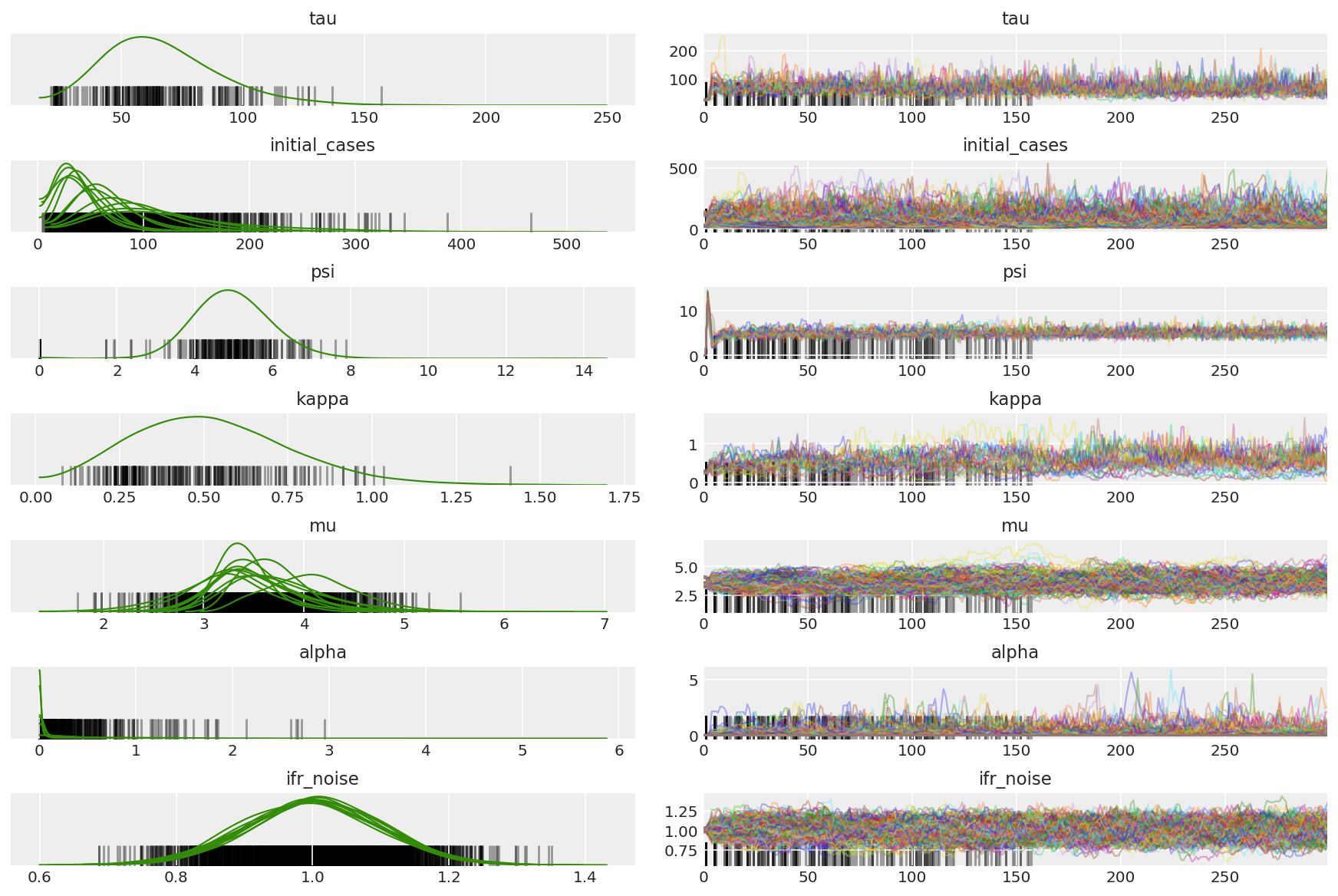
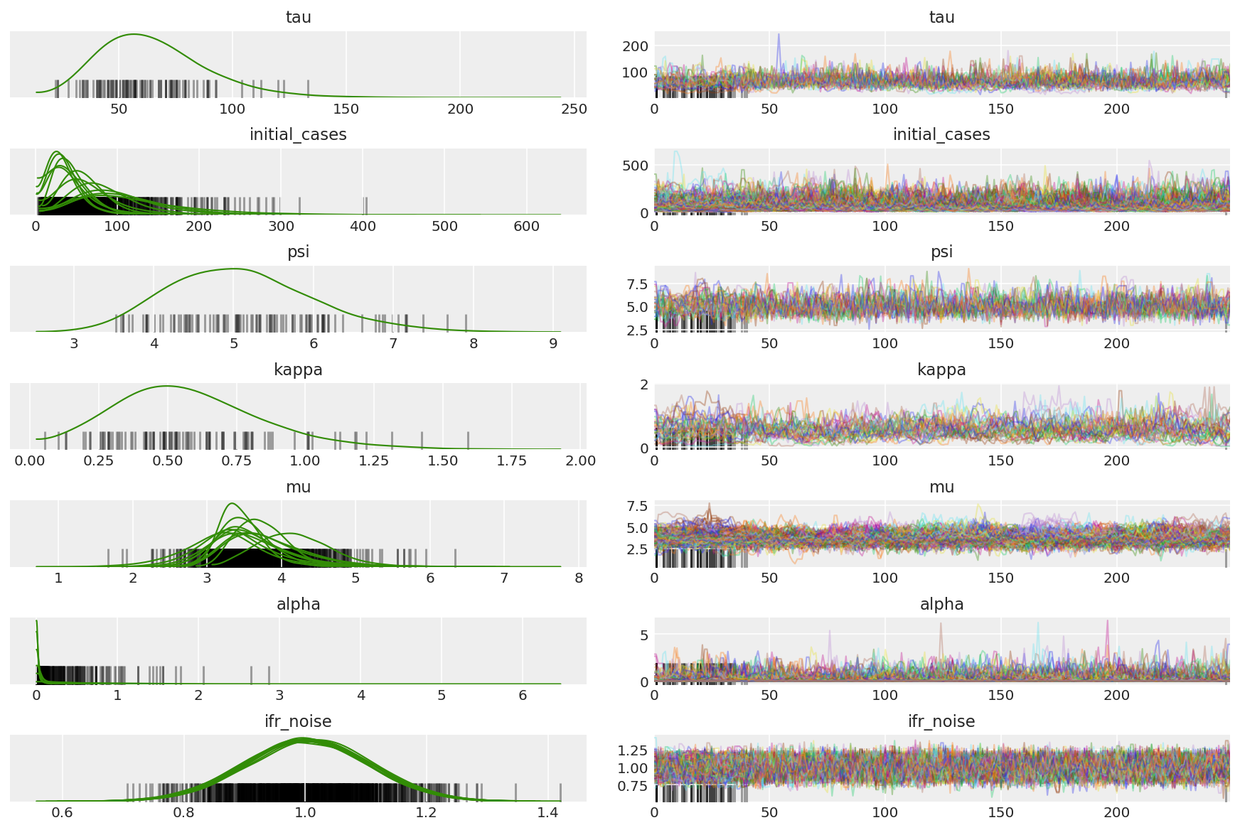
3.5 পাইলট নমুনা কল্পনা করুন
আমরা আটকে থাকা চেইন এবং চক্ষুদানকারী কনভারজেন্স খুঁজছি। আমরা এখানে আনুষ্ঠানিক ডায়াগনস্টিক করতে পারি, তবে এটি শুধুমাত্র একটি পাইলট চালানোর কারণে খুব বেশি প্রয়োজনীয় নয়।
import arviz as az
az.style.use('arviz-darkgrid')
var_name = ['tau', 'initial_cases', 'psi', 'kappa', 'mu', 'alpha', 'ifr_noise']

pilot_with_warmup = {k: np.swapaxes(v.numpy(), 1, 0)
                     for k, v in zip(var_name, pilot_samples)}
আমরা ওয়ার্মআপের সময় ভিন্নতা লক্ষ্য করি, প্রাথমিকভাবে কারণ দ্বৈত গড় ধাপের আকার অভিযোজন সর্বোত্তম ধাপের আকারের জন্য খুব আক্রমণাত্মক অনুসন্ধান ব্যবহার করে। অভিযোজন বন্ধ হয়ে গেলে, ভিন্নতাও অদৃশ্য হয়ে যায়।
az_trace = az.from_dict(posterior=pilot_with_warmup,
                        sample_stats={'diverging': np.swapaxes(pilot_sampler_stat['diverging'].numpy(), 0, 1)})
az.plot_trace(az_trace, combined=True, compact=True, figsize=(12, 8));
plt.plot(pilot_sampler_stat['step_size'][0]);
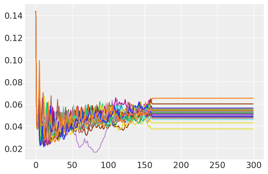
3.6 HMC চালান
নীতিগতভাবে আমরা চূড়ান্ত বিশ্লেষণের জন্য পাইলট নমুনাগুলি ব্যবহার করতে পারি (যদি আমরা এটিকে একত্রিত করার জন্য দীর্ঘ সময় ধরে চালাই), তবে এটি আরেকটি HMC রান শুরু করার জন্য একটু বেশি দক্ষ, এই সময় পূর্বশর্ত এবং পাইলট নমুনা দ্বারা শুরু করা হয়েছে।
%%time

burnin = 50
num_steps = 200

bijectors = get_bijectors_from_samples([s[burnin:] for s in pilot_samples],
                                       unconstraining_bijectors=unconstraining_bijectors,
                                       batch_axes=(0, 1))

samples, sampler_stat = sample_hmc(
    [s[-1] for s in pilot_samples],
    [s[-1] for s in pilot_sampler_stat['step_size']],
    target_log_prob_fn,
    bijectors,
    num_steps=num_steps,
    burnin=burnin,
    num_leapfrog_steps=20)
CPU times: user 1min 26s, sys: 3.88 s, total: 1min 30s
Wall time: 1min 32s
plt.plot(sampler_stat['step_size'][0]);
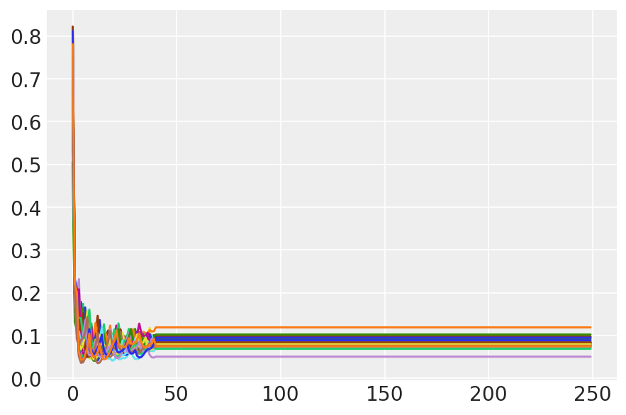
3.7 নমুনা কল্পনা করুন
import arviz as az
az.style.use('arviz-darkgrid')
var_name = ['tau', 'initial_cases', 'psi', 'kappa', 'mu', 'alpha', 'ifr_noise']

posterior = {k: np.swapaxes(v.numpy()[burnin:], 1, 0)
             for k, v in zip(var_name, samples)}
posterior_with_warmup = {k: np.swapaxes(v.numpy(), 1, 0)
             for k, v in zip(var_name, samples)}
চেইনের সারাংশ গণনা করুন। আমরা 1 এর কাছাকাছি উচ্চ ESS এবং r_hat খুঁজছি।
az.summary(posterior)
az_trace = az.from_dict(posterior=posterior_with_warmup,
                        sample_stats={'diverging': np.swapaxes(sampler_stat['diverging'].numpy(), 0, 1)})
az.plot_trace(az_trace, combined=True, compact=True, figsize=(12, 8));
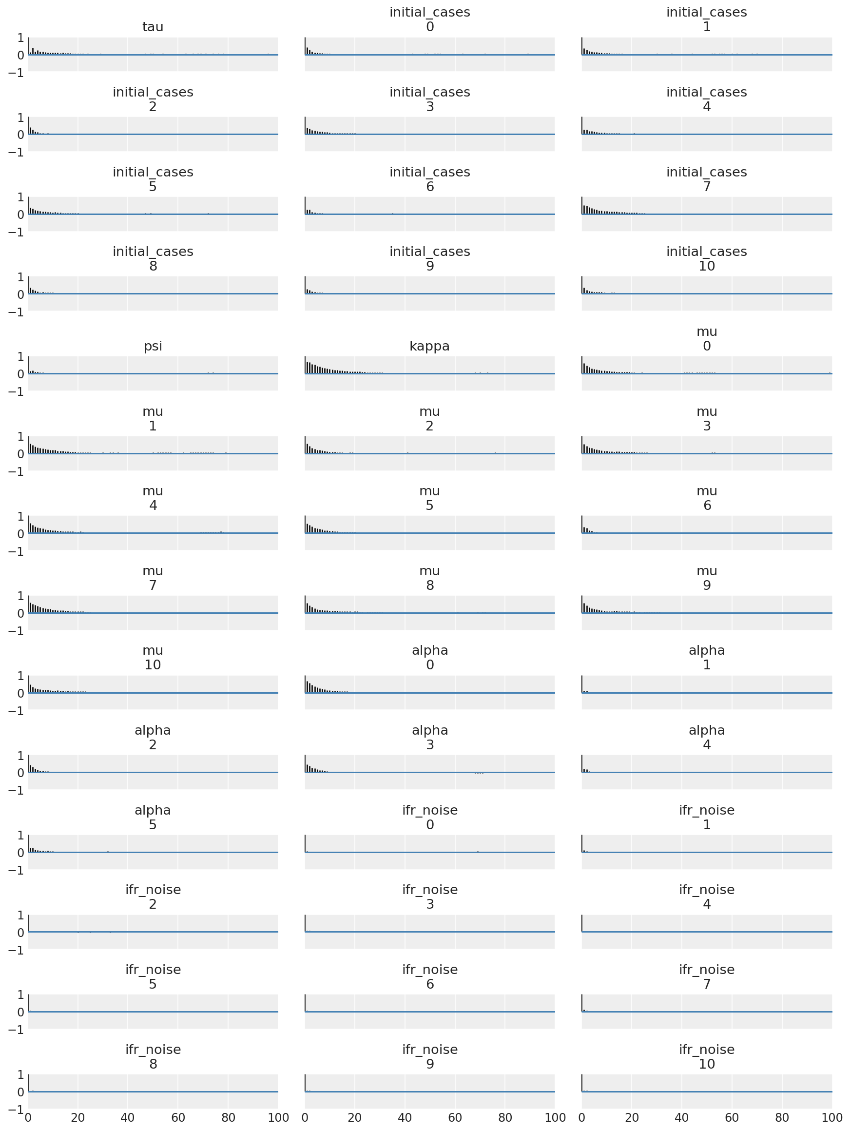
সমস্ত মাত্রা জুড়ে স্বয়ংক্রিয়-সম্পর্কের ফাংশনগুলি দেখার জন্য এটি নির্দেশমূলক। আমরা এমন ফাংশন খুঁজছি যা দ্রুত নেমে যায়, কিন্তু এতটা নয় যে তারা নেতিবাচক দিকে চলে যায় (যা এইচএমসি একটি অনুরণনকে আঘাত করার নির্দেশ করে, যা ergodicity এর জন্য খারাপ এবং পক্ষপাতিত্বের পরিচয় দিতে পারে)।
with az.rc_context(rc={'plot.max_subplots': None}):
  az.plot_autocorr(posterior, combined=True, figsize=(12, 16), textsize=12);
4 ফলাফল
নিম্নলিখিত প্লট উপর অবর ভবিষ্যদ্বাণীপূর্ণ ডিস্ট্রিবিউশন বিশ্লেষণ \(R_t\), মৃত্যুর সংখ্যা, এবং সংক্রমণ, Flaxman এট বিশ্লেষণ অনুরূপ সংখ্যা। (2020)।
total_num_samples = np.prod(posterior['mu'].shape[:2])

# Calculate R_t given parameter estimates.
def rt_samples_batched(mu, intervention_indicators, alpha):
  linear_prediction = tf.reduce_sum(
      intervention_indicators * alpha[..., np.newaxis, np.newaxis, :], axis=-1)
  rt_hat = mu[..., tf.newaxis] * tf.exp(-linear_prediction, name='rt')
  return rt_hat

alpha_hat = tf.convert_to_tensor(
    posterior['alpha'].reshape(total_num_samples, posterior['alpha'].shape[-1]))
mu_hat = tf.convert_to_tensor(
    posterior['mu'].reshape(total_num_samples, num_countries))
rt_hat = rt_samples_batched(mu_hat, intervention_indicators, alpha_hat)
sampled_initial_cases = posterior['initial_cases'].reshape(
    total_num_samples, num_countries)
sampled_ifr_noise = posterior['ifr_noise'].reshape(
    total_num_samples, num_countries)
psi_hat = posterior['psi'].reshape([total_num_samples])

conv_serial_interval = make_conv_serial_interval(INITIAL_DAYS, TOTAL_DAYS)
conv_fatality_rate = make_conv_fatality_rate(infection_fatality_rate, TOTAL_DAYS)
pred_hat = predict_infections(
    intervention_indicators, population_value, sampled_initial_cases, mu_hat,
    alpha_hat, conv_serial_interval, INITIAL_DAYS, TOTAL_DAYS)
expected_deaths = predict_deaths(pred_hat, sampled_ifr_noise, conv_fatality_rate)

psi_m = psi_hat[np.newaxis, ..., np.newaxis]
probs = tf.clip_by_value(expected_deaths / (expected_deaths + psi_m), 1e-9, 1.)
predicted_deaths = tfd.NegativeBinomial(
    total_count=psi_m, probs=probs).sample()
# Predict counterfactual infections/deaths in the absence of interventions
no_intervention_infections = predict_infections(
    intervention_indicators,
    population_value,
    sampled_initial_cases,
    mu_hat,
    tf.zeros_like(alpha_hat),
    conv_serial_interval,
    INITIAL_DAYS, TOTAL_DAYS)

no_intervention_expected_deaths = predict_deaths(
    no_intervention_infections, sampled_ifr_noise, conv_fatality_rate)
probs = tf.clip_by_value(
    no_intervention_expected_deaths / (no_intervention_expected_deaths + psi_m),
    1e-9, 1.)
no_intervention_predicted_deaths = tfd.NegativeBinomial(
    total_count=psi_m, probs=probs).sample()
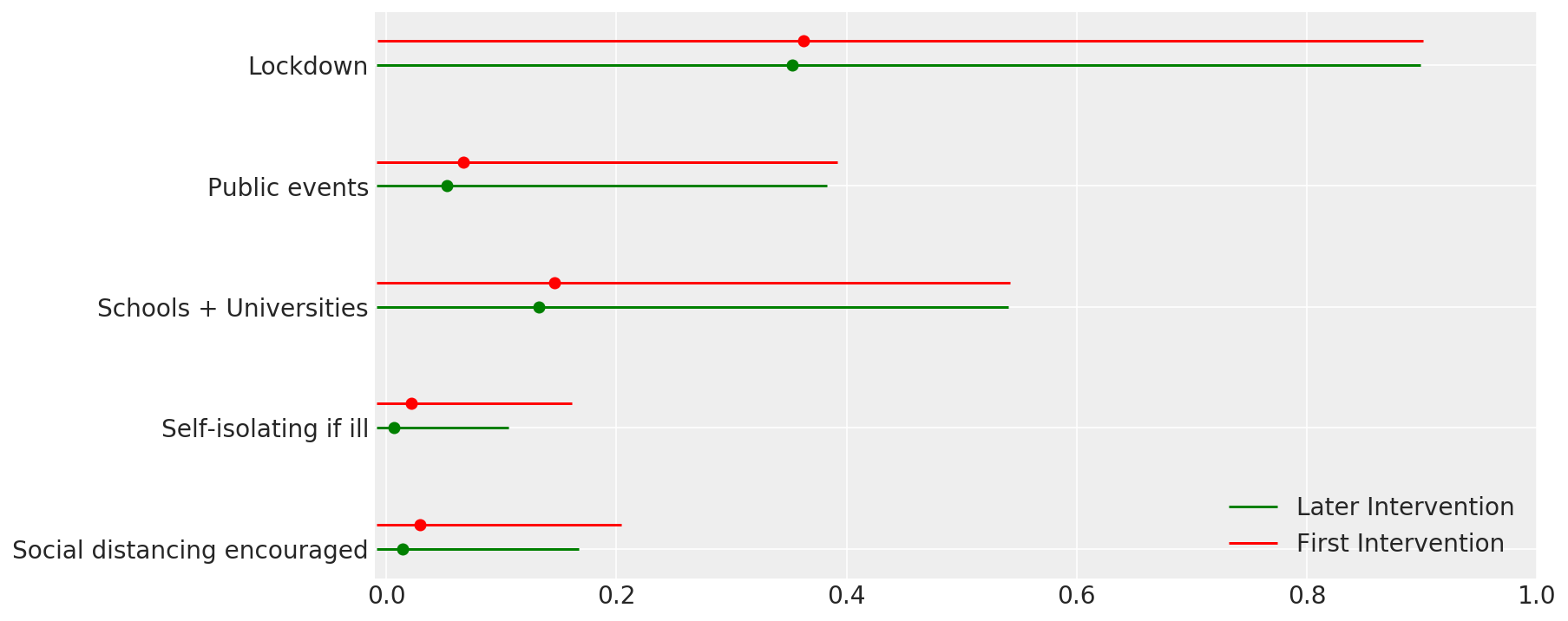
4.1 হস্তক্ষেপের কার্যকারিতা
Flaxman et al এর চিত্র 4 এর অনুরূপ। (2020)।
def intervention_effectiveness(alpha):

  alpha_adj = 1. - np.exp(-alpha + np.log(1.05) / 6.)
  alpha_adj_first = (
      1. - np.exp(-alpha - alpha[..., -1:] + np.log(1.05) / 6.))

  fig, ax = plt.subplots(1, 1, figsize=[12, 6])
  intervention_perm = [2, 1, 3, 4, 0]
  percentile_vals = [2.5, 97.5]
  jitter = .2

  for ind in range(5):
    first_low, first_high = tfp.stats.percentile(
        alpha_adj_first[..., ind], percentile_vals)
    low, high = tfp.stats.percentile(
        alpha_adj[..., ind], percentile_vals)

    p_ind = intervention_perm[ind]
    ax.hlines(p_ind, low, high, label='Later Intervention', colors='g')
    ax.scatter(alpha_adj[..., ind].mean(), p_ind, color='g')
    ax.hlines(p_ind + jitter, first_low, first_high,
              label='First Intervention', colors='r')
    ax.scatter(alpha_adj_first[..., ind].mean(), p_ind + jitter, color='r')

    if ind == 0:
      plt.legend(loc='lower right')
  ax.set_yticks(range(5))
  ax.set_yticklabels(
      [any_intervention_list[intervention_perm.index(p)] for p in range(5)])
  ax.set_xlim([-0.01, 1.])
  r = fig.patch
  r.set_facecolor('white')

intervention_effectiveness(alpha_hat)
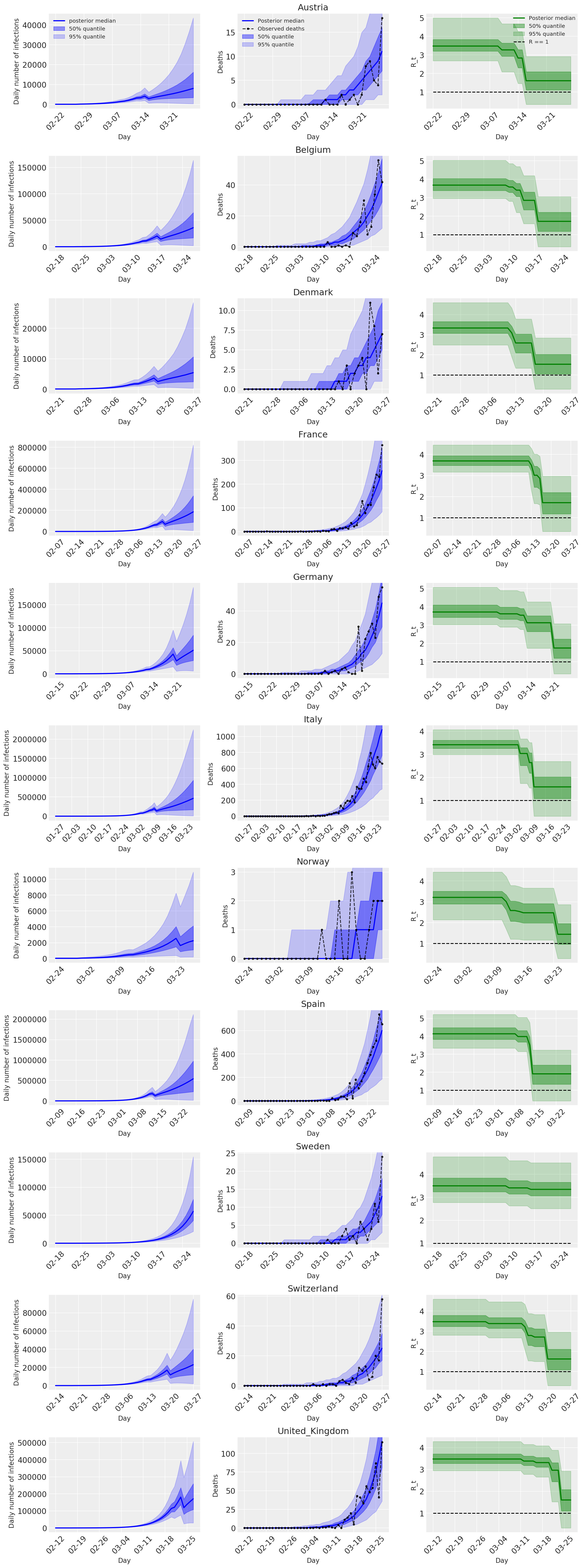
4.2 দেশ অনুসারে সংক্রমণ, মৃত্যু এবং R_t
Flaxman et al এর চিত্র 2 এর অনুরূপ। (2020)।
import matplotlib.dates as mdates

plot_quantile = True
forecast_days = 0

fig, ax = plt.subplots(11, 3, figsize=(15, 40))

for ind, country in enumerate(COUNTRIES):
  num_days = (pd.to_datetime('2020-03-28') - first_days[country]).days + forecast_days
  dates = [(first_days[country] + i*pd.to_timedelta(1, 'days')).strftime('%m-%d') for i in range(num_days)]
  plot_dates = [dates[i] for i in range(0, num_days, 7)]

  # Plot daily number of infections
  infections = pred_hat[:, :, ind]
  posterior_quantile = np.percentile(infections, [2.5, 25, 50, 75, 97.5], axis=-1)
  ax[ind, 0].plot(
      dates, posterior_quantile[2, :num_days],
      color='b', label='posterior median', lw=2)
  if plot_quantile:
    ax[ind, 0].fill_between(
        dates, posterior_quantile[1, :num_days], posterior_quantile[3, :num_days],
        color='b', label='50% quantile', alpha=.4)
    ax[ind, 0].fill_between(
        dates, posterior_quantile[0, :num_days], posterior_quantile[4, :num_days],
        color='b', label='95% quantile', alpha=.2)

  ax[ind, 0].set_xticks(plot_dates)
  ax[ind, 0].xaxis.set_tick_params(rotation=45)
  ax[ind, 0].set_ylabel('Daily number of infections', fontsize='large')
  ax[ind, 0].set_xlabel('Day', fontsize='large')

  # Plot deaths
  ax[ind, 1].set_title(country)

  samples = predicted_deaths[:, :, ind]
  posterior_quantile = np.percentile(samples, [2.5, 25, 50, 75, 97.5], axis=-1)
  ax[ind, 1].plot(
      range(num_days), posterior_quantile[2, :num_days],
      color='b', label='Posterior median', lw=2)
  if plot_quantile:
    ax[ind, 1].fill_between(
        range(num_days), posterior_quantile[1, :num_days], posterior_quantile[3, :num_days],
        color='b', label='50% quantile', alpha=.4)
    ax[ind, 1].fill_between(
        range(num_days), posterior_quantile[0, :num_days], posterior_quantile[4, :num_days],
        color='b', label='95% quantile', alpha=.2)

  observed = deaths[ind, :]
  observed[observed == -1] = np.nan
  ax[ind, 1].plot(
      dates, observed[:num_days],
      '--o', color='k', markersize=3,
      label='Observed deaths', alpha=.8)
  ax[ind, 1].set_xticks(plot_dates)
  ax[ind, 1].xaxis.set_tick_params(rotation=45)
  ax[ind, 1].set_title(country)
  ax[ind, 1].set_xlabel('Day', fontsize='large')
  ax[ind, 1].set_ylabel('Deaths', fontsize='large')

  # Plot R_t
  samples = np.transpose(rt_hat[:, ind, :])
  posterior_quantile = np.percentile(samples, [2.5, 25, 50, 75, 97.5], axis=-1)
  l1 = ax[ind, 2].plot(
      dates, posterior_quantile[2, :num_days],
      color='g', label='Posterior median', lw=2)
  l2 = ax[ind, 2].fill_between(
      dates, posterior_quantile[1, :num_days], posterior_quantile[3, :num_days],
      color='g', label='50% quantile', alpha=.4)
  if plot_quantile:
    l3 = ax[ind, 2].fill_between(
        dates, posterior_quantile[0, :num_days], posterior_quantile[4, :num_days],
        color='g', label='95% quantile', alpha=.2)

  l4 = ax[ind, 2].hlines(1., dates[0], dates[-1], linestyle='--', label='R == 1')
  ax[ind, 2].set_xlabel('Day', fontsize='large')
  ax[ind, 2].set_ylabel('R_t', fontsize='large')
  ax[ind, 2].set_xticks(plot_dates)
  ax[ind, 2].xaxis.set_tick_params(rotation=45)

fontsize = 'medium'
ax[0, 0].legend(loc='upper left', fontsize=fontsize)
ax[0, 1].legend(loc='upper left', fontsize=fontsize)
ax[0, 2].legend(
  bbox_to_anchor=(1., 1.),
  loc='upper right',
  borderaxespad=0.,
  fontsize=fontsize)

plt.tight_layout();
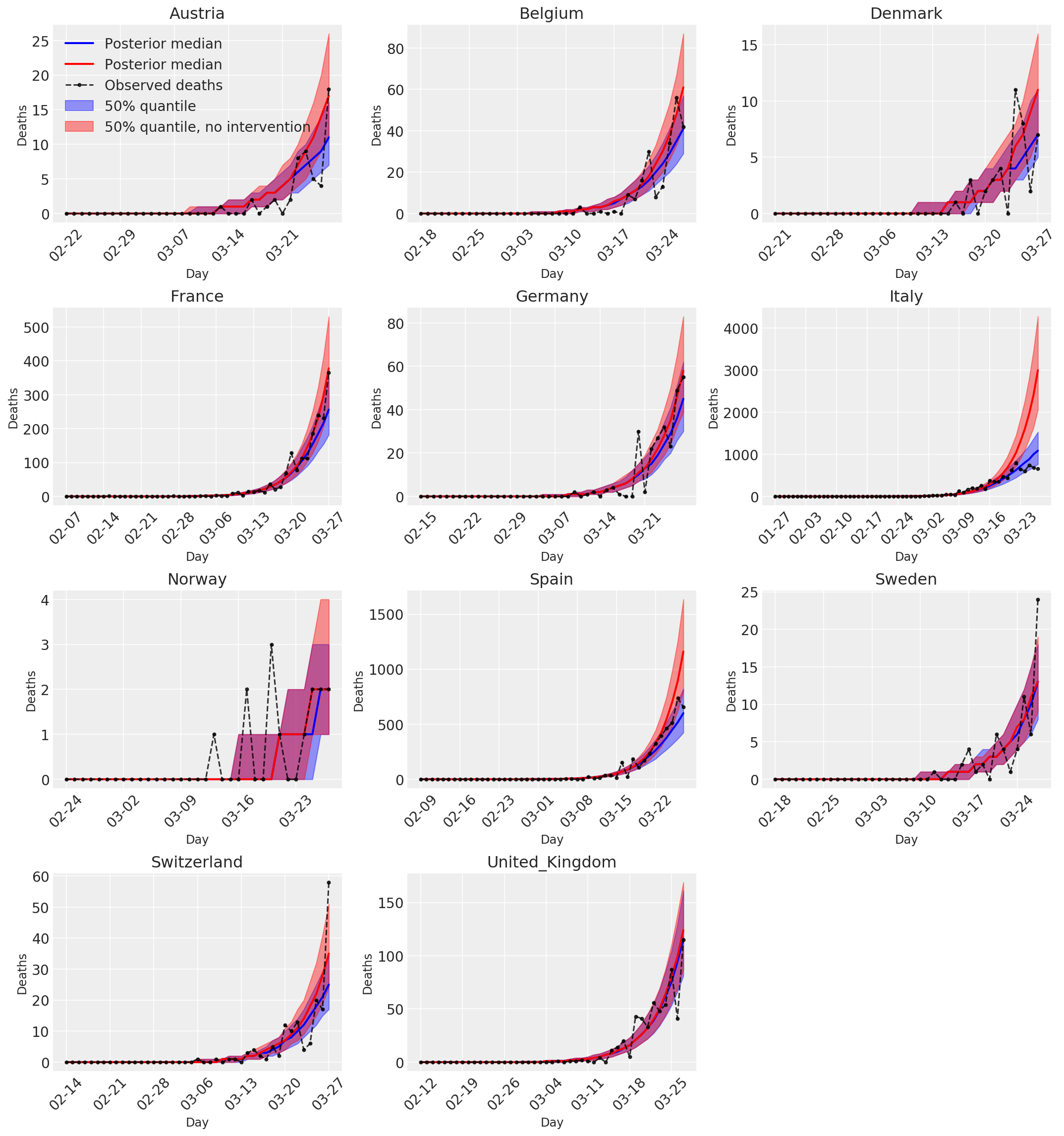
4.3 হস্তক্ষেপ সহ এবং ছাড়াই পূর্বাভাসিত/পূর্বাভাসিত মৃত্যুর দৈনিক সংখ্যা
plot_quantile = True
forecast_days = 0

fig, ax = plt.subplots(4, 3, figsize=(15, 16))
ax = ax.flatten()
fig.delaxes(ax[-1])
for country_index, country in enumerate(COUNTRIES):
  num_days = (pd.to_datetime('2020-03-28') - first_days[country]).days + forecast_days
  dates = [(first_days[country] + i*pd.to_timedelta(1, 'days')).strftime('%m-%d') for i in range(num_days)]
  plot_dates = [dates[i] for i in range(0, num_days, 7)]

  ax[country_index].set_title(country)

  quantile_vals = [.025, .25, .5, .75, .975]
  samples = predicted_deaths[:, :, country_index].numpy()
  quantiles = []

  psi_m = psi_hat[np.newaxis, ..., np.newaxis]
  probs = tf.clip_by_value(expected_deaths / (expected_deaths + psi_m), 1e-9, 1.)
  predicted_deaths_dist = tfd.NegativeBinomial(
    total_count=psi_m, probs=probs)

  posterior_quantile = np.percentile(samples, [2.5, 25, 50, 75, 97.5], axis=-1)
  ax[country_index].plot(
      dates, posterior_quantile[2, :num_days],
      color='b', label='Posterior median', lw=2)
  if plot_quantile:
    ax[country_index].fill_between(
        dates, posterior_quantile[1, :num_days], posterior_quantile[3, :num_days],
        color='b', label='50% quantile', alpha=.4)

  samples_counterfact = no_intervention_predicted_deaths[:, :, country_index]
  posterior_quantile = np.percentile(samples_counterfact, [2.5, 25, 50, 75, 97.5], axis=-1)
  ax[country_index].plot(
      dates, posterior_quantile[2, :num_days],
      color='r', label='Posterior median', lw=2)
  if plot_quantile:
    ax[country_index].fill_between(
        dates, posterior_quantile[1, :num_days], posterior_quantile[3, :num_days],
        color='r', label='50% quantile, no intervention', alpha=.4)

  observed = deaths[country_index, :]
  observed[observed == -1] = np.nan
  ax[country_index].plot(
      dates, observed[:num_days],
      '--o', color='k', markersize=3,
      label='Observed deaths', alpha=.8)
  ax[country_index].set_xticks(plot_dates)
  ax[country_index].xaxis.set_tick_params(rotation=45)
  ax[country_index].set_title(country)
  ax[country_index].set_xlabel('Day', fontsize='large')
  ax[country_index].set_ylabel('Deaths', fontsize='large')
  ax[0].legend(loc='upper left')
plt.tight_layout(pad=1.0);