หน้านี้ได้รับการแปลโดย Cloud Translation API

การสร้างแบบจำลอง COVID-19 แพร่กระจายในยุโรปและผลกระทบของการแทรกแซง

ได้รับใบอนุญาตภายใต้ใบอนุญาต MIT

# Permission is hereby granted, free of charge, to any person obtaining a copy
# of this software and associated documentation files (the "Software"), to deal
# in the Software without restriction, including without limitation the rights
# to use, copy, modify, merge, publish, distribute, sublicense, and/or sell
# copies of the Software, and to permit persons to whom the Software is
# furnished to do so, subject to the following conditions:
#
# The above copyright notice and this permission notice shall be included in all
# copies or substantial portions of the Software.
#
# THE SOFTWARE IS PROVIDED "AS IS", WITHOUT WARRANTY OF ANY KIND, EXPRESS OR
# IMPLIED, INCLUDING BUT NOT LIMITED TO THE WARRANTIES OF MERCHANTABILITY,
# FITNESS FOR A PARTICULAR PURPOSE AND NONINFRINGEMENT. IN NO EVENT SHALL THE
# AUTHORS OR COPYRIGHT HOLDERS BE LIABLE FOR ANY CLAIM, DAMAGES OR OTHER
# LIABILITY, WHETHER IN AN ACTION OF CONTRACT, TORT OR OTHERWISE, ARISING FROM,
# OUT OF OR IN CONNECTION WITH THE SOFTWARE OR THE USE OR OTHER DEALINGS IN THE
# SOFTWARE.

ดูบน TensorFlow.org

ทำงานใน Google Colab

ดูแหล่งที่มาบน GitHub

ดาวน์โหลดโน๊ตบุ๊ค

เพื่อชะลอการแพร่กระจายของ COVID-19 ในต้นปี 2020 ประเทศต่างๆ ในยุโรปได้นำมาตรการที่ไม่ใช้เภสัชภัณฑ์มาใช้ เช่น การปิดธุรกิจที่ไม่จำเป็น การแยกแต่ละกรณี การห้ามเดินทาง และมาตรการอื่นๆ เพื่อสนับสนุนการเว้นระยะห่างทางสังคม การตอบสนองของทีมอิมพีเรียลคอลเลจ COVID-19 การวิเคราะห์ประสิทธิภาพของมาตรการเหล่านี้ในกระดาษของพวกเขา "ประมาณจำนวนผู้ติดเชื้อและผลกระทบของการแทรกแซงที่ไม่ใช่ยาใน COVID-19 ใน 11 ประเทศยุโรป" โดยใช้แบบลำดับชั้นแบบเบย์รวมกับกลไก แบบจำลองทางระบาดวิทยา

Colab นี้มีการนำ TensorFlow Probability (TFP) ไปใช้ของการวิเคราะห์นั้น ซึ่งจัดเป็นดังนี้:

"การตั้งค่าแบบจำลอง" กำหนดแบบจำลองทางระบาดวิทยาสำหรับการแพร่กระจายของโรคและการเสียชีวิตที่เป็นผล การกระจายก่อนหน้าแบบเบย์เซียนเหนือพารามิเตอร์แบบจำลอง และการกระจายของจำนวนผู้เสียชีวิตตามเงื่อนไขบนค่าพารามิเตอร์
"การประมวลผลข้อมูลล่วงหน้า" จะโหลดข้อมูลเกี่ยวกับเวลาและประเภทของการแทรกแซงในแต่ละประเทศ จำนวนผู้เสียชีวิตในช่วงเวลาหนึ่ง และอัตราการเสียชีวิตโดยประมาณของผู้ติดเชื้อ
"การอนุมานแบบจำลอง" จะสร้างแบบจำลองลำดับชั้นแบบเบย์และเรียกใช้ Hamiltonian Monte Carlo (HMC) เพื่อสุ่มตัวอย่างจากการแจกแจงภายหลังเหนือพารามิเตอร์
"ผลลัพธ์" แสดงการแจกแจงแบบคาดการณ์ภายหลังสำหรับปริมาณที่น่าสนใจ เช่น จำนวนผู้เสียชีวิตที่คาดการณ์ และการเสียชีวิตจากข้อเท็จจริงในกรณีที่ไม่มีการแทรกแซง

กระดาษพบหลักฐานว่าประเทศที่มีการจัดการเพื่อลดจำนวนผู้ติดเชื้อใหม่ส่งโดยแต่ละคนที่ติดเชื้อ (คน $R_t$ ) แต่ที่ช่วงเวลาที่มีความน่าเชื่อถือมี $R_t=1$ (ราคาดังกล่าวข้างต้นซึ่งการแพร่ระบาดยังคงแพร่กระจาย) และว่ามันเป็นก่อนวัยอันควร เพื่อหาข้อสรุปที่ชัดเจนเกี่ยวกับประสิทธิผลของการแทรกแซง รหัสสแตนสำหรับกระดาษที่อยู่ในผู้เขียน Github พื้นที่เก็บข้อมูลและ Colab นี้พันธุ์ รุ่นที่ 2

pip3 install -q git+git://github.com/arviz-devs/arviz.git
pip3 install -q tf-nightly tfp-nightly

นำเข้า

import collections
from pprint import pprint

import numpy as np
import pandas as pd

import matplotlib.pyplot as plt

%config InlineBackend.figure_format = 'retina'

import tensorflow.compat.v2 as tf
import tensorflow_probability as tfp
from tensorflow_probability.python.internal import prefer_static as ps

tf.enable_v2_behavior()

# Globally Enable XLA.
# tf.config.optimizer.set_jit(True)

try:
  physical_devices = tf.config.list_physical_devices('GPU')
  tf.config.experimental.set_memory_growth(physical_devices[0], True)
except:
  # Invalid device or cannot modify virtual devices once initialized.
  pass

tfb = tfp.bijectors
tfd = tfp.distributions

DTYPE = np.float32

1 การติดตั้งโมเดล

1.1 แบบจำลองกลไกการติดเชื้อและการเสียชีวิต

โมเดลการติดเชื้อจะจำลองจำนวนผู้ติดเชื้อในแต่ละประเทศในช่วงเวลาหนึ่ง ข้อมูลที่ป้อนเข้าคือเวลาและประเภทของการแทรกแซง ขนาดประชากร และกรณีเริ่มต้น พารามิเตอร์ควบคุมประสิทธิผลของการแทรกแซงและอัตราการแพร่โรค แบบจำลองสำหรับจำนวนผู้เสียชีวิตที่คาดไว้ใช้อัตราการเสียชีวิตกับการติดเชื้อที่คาดการณ์ไว้

แบบจำลองการติดเชื้อดำเนินการแปลงการติดเชื้อรายวันก่อนหน้าด้วยการแจกจ่ายช่วงเวลาต่อเนื่อง (การกระจายตามจำนวนวันที่ติดเชื้อและการแพร่เชื้อของผู้อื่น) ในแต่ละขั้นตอนเวลาจำนวนผู้ติดเชื้อใหม่ในเวลา $t$ , $n_t$ , คำนวณเป็น

\begin{equation} \sum_{i=0}^{t-1} n_i \mu_t \text{p} (\text{จับจากคนที่ติดเชื้อที่ } i | \text{ติดเชื้อใหม่ที่ } t) \end{ สม} ที่ $\mu_t=R_t$ และน่าจะเป็นเงื่อนไขถูกเก็บไว้ใน conv_serial_interval ที่กำหนดไว้ด้านล่าง

แบบจำลองสำหรับการเสียชีวิตที่คาดหวังทำให้เกิดการติดเชื้อรายวันและการกระจายของวันระหว่างการติดเชื้อและการเสียชีวิต นั่นคือการเสียชีวิตคาดว่าในวัน $t$ คำนวณเป็น

\ begin {สม} \ sum_ {i = 0} ^ {t-1} n_i \ ข้อความ {p (ตายในวัน $t$ | การติดเชื้อในวัน $i$ )} \ end {สม} ที่น่าจะเป็นเงื่อนไขจะถูกเก็บไว้ ใน conv_fatality_rate ที่กำหนดไว้ด้านล่าง

from tensorflow_probability.python.internal import broadcast_util as bu

def predict_infections(
    intervention_indicators, population, initial_cases, mu, alpha_hier,
    conv_serial_interval, initial_days, total_days):
  """Predict the number of infections by forward-simulation.

  Args:
    intervention_indicators: Binary array of shape
      `[num_countries, total_days, num_interventions]`, in which `1` indicates
      the intervention is active in that country at that time and `0` indicates
      otherwise.
    population: Vector of length `num_countries`. Population of each country.
    initial_cases: Array of shape `[batch_size, num_countries]`. Number of cases
      in each country at the start of the simulation.
    mu: Array of shape `[batch_size, num_countries]`. Initial reproduction rate
      (R_0) by country.
    alpha_hier: Array of shape `[batch_size, num_interventions]` representing
      the effectiveness of interventions.
    conv_serial_interval: Array of shape
      `[total_days - initial_days, total_days]` output from
      `make_conv_serial_interval`. Convolution kernel for serial interval
      distribution.
    initial_days: Integer, number of sequential days to seed infections after
      the 10th death in a country. (N0 in the authors' Stan code.)
    total_days: Integer, number of days of observed data plus days to forecast.
      (N2 in the authors' Stan code.)
  Returns:
    predicted_infections: Array of shape
      `[total_days, batch_size, num_countries]`. (Batched) predicted number of
      infections over time and by country.
  """
  alpha = alpha_hier - tf.cast(np.log(1.05) / 6.0, DTYPE)

  # Multiply the effectiveness of each intervention in each country (alpha)
  # by the indicator variable for whether the intervention was active and sum
  # over interventions, yielding an array of shape
  # [total_days, batch_size, num_countries] that represents the total effectiveness of
  # all interventions in each country on each day (for a batch of data).
  linear_prediction = tf.einsum(
      'ijk,...k->j...i', intervention_indicators, alpha)

  # Adjust the reproduction rate per country downward, according to the
  # effectiveness of the interventions.
  rt = mu * tf.exp(-linear_prediction, name='reproduction_rate')

  # Initialize storage array for daily infections and seed it with initial
  # cases.
  daily_infections = tf.TensorArray(
      dtype=DTYPE, size=total_days, element_shape=initial_cases.shape)
  for i in range(initial_days):
    daily_infections = daily_infections.write(i, initial_cases)

  # Initialize cumulative cases.
  init_cumulative_infections = initial_cases * initial_days

  # Simulate forward for total_days days.
  cond = lambda i, *_: i < total_days
  def body(i, prev_daily_infections, prev_cumulative_infections):
    # The probability distribution over days j that someone infected on day i
    # caught the virus from someone infected on day j.
    p_infected_on_day = tf.gather(
        conv_serial_interval, i - initial_days, axis=0)

    # Multiply p_infected_on_day by the number previous infections each day and
    # by mu, and sum to obtain new infections on day i. Mu is adjusted by
    # the fraction of the population already infected, so that the population
    # size is the upper limit on the number of infections.
    prev_daily_infections_array = prev_daily_infections.stack()
    to_sum = prev_daily_infections_array * bu.left_justified_expand_dims_like(
        p_infected_on_day, prev_daily_infections_array)
    convolution = tf.reduce_sum(to_sum, axis=0)
    rt_adj = (
        (population - prev_cumulative_infections) / population
        ) * tf.gather(rt, i)
    new_infections = rt_adj * convolution

    # Update the prediction array and the cumulative number of infections.
    daily_infections = prev_daily_infections.write(i, new_infections)
    cumulative_infections = prev_cumulative_infections + new_infections
    return i + 1, daily_infections, cumulative_infections

  _, daily_infections_final, last_cumm_sum = tf.while_loop(
      cond, body,
      (initial_days, daily_infections, init_cumulative_infections),
      maximum_iterations=(total_days - initial_days))
  return daily_infections_final.stack()

def predict_deaths(predicted_infections, ifr_noise, conv_fatality_rate):
  """Expected number of reported deaths by country, by day.

  Args:
    predicted_infections: Array of shape
      `[total_days, batch_size, num_countries]` output from
      `predict_infections`.
    ifr_noise: Array of shape `[batch_size, num_countries]`. Noise in Infection
      Fatality Rate (IFR).
    conv_fatality_rate: Array of shape
      `[total_days - 1, total_days, num_countries]`. Convolutional kernel for
      calculating fatalities, output from `make_conv_fatality_rate`.
  Returns:
    predicted_deaths: Array of shape `[total_days, batch_size, num_countries]`.
      (Batched) predicted number of deaths over time and by country.
  """
  # Multiply the number of infections on day j by the probability of death
  # on day i given infection on day j, and sum over j. This yields the expected
  result_remainder = tf.einsum(
      'i...j,kij->k...j', predicted_infections, conv_fatality_rate) * ifr_noise

  # Concatenate the result with a vector of zeros so that the first day is
  # included.
  result_temp = 1e-15 * predicted_infections[:1]
  return tf.concat([result_temp, result_remainder], axis=0)

1.2 ก่อนหน้าค่าพารามิเตอร์

ที่นี่เรากำหนดการกระจายก่อนหน้าร่วมกันเหนือพารามิเตอร์แบบจำลอง ค่าพารามิเตอร์หลายค่าถือว่าเป็นอิสระ ดังนั้นค่าก่อนหน้าสามารถแสดงเป็น:

$\text p(\tau, y, \psi, \kappa, \mu, \alpha) = \text p(\tau)\text p(y|\tau)\text p(\psi)\text p(\kappa)\text p(\mu|\kappa)\text p(\alpha)\text p(\epsilon)$

ซึ่งใน:

$\tau$ คือพารามิเตอร์อัตราการใช้ร่วมกันของการกระจายชี้แจงมากกว่าจำนวนผู้ป่วยเริ่มต้นต่อประเทศ $y = y_1, ... y_{\text{num_countries} }$
$\psi$ เป็นพารามิเตอร์ในการกระจายทวินามเชิงลบสำหรับจำนวนของการเสียชีวิต
$\kappa$ คือพารามิเตอร์ขนาดที่ใช้ร่วมกันของการกระจาย HalfNormal มากกว่าจำนวนการสืบพันธุ์เริ่มต้นในแต่ละประเทศ $\mu = \mu_1, ..., \mu_{\text{num_countries} }$ (ระบุจำนวนผู้ป่วยที่เพิ่มขึ้นส่งโดยแต่ละคนที่ติดเชื้อ)
$\alpha = \alpha_1, ..., \alpha_6$ คือประสิทธิผลของแต่ละหกแทรกแซง
$\epsilon$ (เรียกว่า ifr_noise ในรหัสหลังจากที่ผู้เขียนรหัสแตน) เป็นเสียงในการติดเชื้อตาย Rate (IFR)

เราแสดงโมเดลนี้ว่าเป็น TFP JointDistribution ซึ่งเป็นประเภทของการกระจาย TFP ที่ช่วยให้สามารถแสดงรูปแบบกราฟิกที่น่าจะเป็นได้

def make_jd_prior(num_countries, num_interventions):
  return tfd.JointDistributionSequentialAutoBatched([
      # Rate parameter for the distribution of initial cases (tau).
      tfd.Exponential(rate=tf.cast(0.03, DTYPE)),

      # Initial cases for each country.
      lambda tau: tfd.Sample(
          tfd.Exponential(rate=tf.cast(1, DTYPE) / tau),
          sample_shape=num_countries),

      # Parameter in Negative Binomial model for deaths (psi).
      tfd.HalfNormal(scale=tf.cast(5, DTYPE)),

      # Parameter in the distribution over the initial reproduction number, R_0
      # (kappa).
      tfd.HalfNormal(scale=tf.cast(0.5, DTYPE)),

      # Initial reproduction number, R_0, for each country (mu).
      lambda kappa: tfd.Sample(
          tfd.TruncatedNormal(loc=3.28, scale=kappa, low=1e-5, high=1e5),
          sample_shape=num_countries),

      # Impact of interventions (alpha; shared for all countries).
      tfd.Sample(
          tfd.Gamma(tf.cast(0.1667, DTYPE), 1), sample_shape=num_interventions),

      # Multiplicative noise in Infection Fatality Rate.
      tfd.Sample(
          tfd.TruncatedNormal(
              loc=tf.cast(1., DTYPE), scale=0.1, low=1e-5, high=1e5),
              sample_shape=num_countries)
  ])

1.3 ความน่าจะเป็นของการเสียชีวิตที่สังเกตได้โดยมีเงื่อนไขตามค่าพารามิเตอร์

รูปแบบความน่าจะเป็นการแสดงออกถึงความ $p(\text{deaths} | \tau, y, \psi, \kappa, \mu, \alpha, \epsilon)$ ใช้แบบจำลองสำหรับจำนวนการติดเชื้อและการเสียชีวิตที่คาดหวังตามเงื่อนไขของพารามิเตอร์ และถือว่าการเสียชีวิตจริงเป็นไปตามการแจกแจงทวินามเชิงลบ

def make_likelihood_fn(
    intervention_indicators, population, deaths,
    infection_fatality_rate, initial_days, total_days):

  # Create a mask for the initial days of simulated data, as they are not
  # counted in the likelihood.
  observed_deaths = tf.constant(deaths.T[np.newaxis, ...], dtype=DTYPE)
  mask_temp = deaths != -1
  mask_temp[:, :START_DAYS] = False
  observed_deaths_mask = tf.constant(mask_temp.T[np.newaxis, ...])

  conv_serial_interval = make_conv_serial_interval(initial_days, total_days)
  conv_fatality_rate = make_conv_fatality_rate(
      infection_fatality_rate, total_days)

  def likelihood_fn(tau, initial_cases, psi, kappa, mu, alpha_hier, ifr_noise):
    # Run models for infections and expected deaths
    predicted_infections = predict_infections(
        intervention_indicators, population, initial_cases, mu, alpha_hier,
        conv_serial_interval, initial_days, total_days)
    e_deaths_all_countries = predict_deaths(
        predicted_infections, ifr_noise, conv_fatality_rate)

    # Construct the Negative Binomial distribution for deaths by country.
    mu_m = tf.transpose(e_deaths_all_countries, [1, 0, 2])
    psi_m = psi[..., tf.newaxis, tf.newaxis]
    probs = tf.clip_by_value(mu_m / (mu_m + psi_m), 1e-9, 1.)
    likelihood_elementwise = tfd.NegativeBinomial(
        total_count=psi_m, probs=probs).log_prob(observed_deaths)
    return tf.reduce_sum(
        tf.where(observed_deaths_mask,
                likelihood_elementwise,
                tf.zeros_like(likelihood_elementwise)),
        axis=[-2, -1])

  return likelihood_fn

1.4 ความน่าจะเป็นของการเสียชีวิตจากการติดเชื้อ

ส่วนนี้คำนวณการกระจายการเสียชีวิตในวันหลังการติดเชื้อ ถือว่าเวลาตั้งแต่ติดเชื้อจนตายเป็นผลรวมของปริมาณตัวแปรแกมมาสองปริมาณ ซึ่งแทนเวลาตั้งแต่การติดเชื้อจนถึงเริ่มมีโรค และเวลาตั้งแต่เริ่มมีอาการจนถึงตาย มีการกระจายของเวลาในการตายจะถูกรวมกับการติดเชื้อข้อมูลอัตราการตายจาก ความแม่นยำ, et al (2020) ในการคำนวณความน่าจะเป็นของการเสียชีวิตในวันต่อไปนี้การติดเชื้อ

def daily_fatality_probability(infection_fatality_rate, total_days):
  """Computes the probability of death `d` days after infection."""

  # Convert from alternative Gamma parametrization and construct distributions
  # for number of days from infection to onset and onset to death.
  concentration1 = tf.cast((1. / 0.86)**2, DTYPE)
  rate1 = concentration1 / 5.1
  concentration2 = tf.cast((1. / 0.45)**2, DTYPE)
  rate2 = concentration2 / 18.8
  infection_to_onset = tfd.Gamma(concentration=concentration1, rate=rate1)
  onset_to_death = tfd.Gamma(concentration=concentration2, rate=rate2)

  # Create empirical distribution for number of days from infection to death.
  inf_to_death_dist = tfd.Empirical(
      infection_to_onset.sample([5e6]) + onset_to_death.sample([5e6]))

  # Subtract the CDF value at day i from the value at day i + 1 to compute the
  # probability of death on day i given infection on day 0, and given that
  # death (not recovery) is the outcome.
  times = np.arange(total_days + 1., dtype=DTYPE) + 0.5
  cdf = inf_to_death_dist.cdf(times).numpy()
  f_before_ifr = cdf[1:] - cdf[:-1]
  # Explicitly set the zeroth value to the empirical cdf at time 1.5, to include
  # the mass between time 0 and time .5.
  f_before_ifr[0] = cdf[1]

  # Multiply the daily fatality rates conditional on infection and eventual
  # death (f_before_ifr) by the infection fatality rates (probability of death
  # given intection) to obtain the probability of death on day i conditional
  # on infection on day 0.
  return infection_fatality_rate[..., np.newaxis] * f_before_ifr

def make_conv_fatality_rate(infection_fatality_rate, total_days):
  """Computes the probability of death on day `i` given infection on day `j`."""
  p_fatal_all_countries = daily_fatality_probability(
      infection_fatality_rate, total_days)

  # Use the probability of death d days after infection in each country
  # to build an array of shape [total_days - 1, total_days, num_countries],
  # where the element [i, j, c] is the probability of death on day i+1 given
  # infection on day j in country c.
  conv_fatality_rate = np.zeros(
      [total_days - 1, total_days, p_fatal_all_countries.shape[0]])
  for n in range(1, total_days):
    conv_fatality_rate[n - 1, 0:n, :] = (
        p_fatal_all_countries[:, n - 1::-1]).T
  return tf.constant(conv_fatality_rate, dtype=DTYPE)

1.5 ช่วงเวลาอนุกรม

ช่วงเวลาต่อเนื่องกันคือเวลาระหว่างกรณีต่างๆ ที่ต่อเนื่องกันในสายการแพร่ของโรค และถือว่ามีการกระจายแกมมา เราใช้การกระจายอนุกรมช่วงเวลาในการคำนวณความน่าจะเป็นว่าคนที่ติดเชื้อในวัน $i$ จับไวรัสจากคนที่ติดเชื้อก่อนหน้านี้ในวันที่ $j$ (คน conv_serial_interval อาร์กิวเมนต์ predict_infections )

def make_conv_serial_interval(initial_days, total_days):
  """Construct the convolutional kernel for infection timing."""

  g = tfd.Gamma(tf.cast(1. / (0.62**2), DTYPE), 1./(6.5*0.62**2))
  g_cdf = g.cdf(np.arange(total_days, dtype=DTYPE))

  # Approximate the probability mass function for the number of days between
  # successive infections.
  serial_interval = g_cdf[1:] - g_cdf[:-1]

  # `conv_serial_interval` is an array of shape
  # [total_days - initial_days, total_days] in which entry [i, j] contains the
  # probability that an individual infected on day i + initial_days caught the
  # virus from someone infected on day j.
  conv_serial_interval = np.zeros([total_days - initial_days, total_days])
  for n in range(initial_days, total_days):
    conv_serial_interval[n - initial_days, 0:n] = serial_interval[n - 1::-1]
  return tf.constant(conv_serial_interval, dtype=DTYPE)

2 การประมวลผลข้อมูลล่วงหน้า

COUNTRIES = [
    'Austria',
    'Belgium',
    'Denmark',
    'France',
    'Germany',
    'Italy',
    'Norway',
    'Spain',
    'Sweden',
    'Switzerland',
    'United_Kingdom'
]

2.1 ดึงข้อมูลและประมวลผลข้อมูลล่วงหน้า

raw_interventions = pd.read_csv(
    'https://raw.githubusercontent.com/ImperialCollegeLondon/covid19model/master/data/interventions.csv')

raw_interventions['Date effective'] = pd.to_datetime(
    raw_interventions['Date effective'], dayfirst=True)
interventions = raw_interventions.pivot(index='Country', columns='Type', values='Date effective')

# If any interventions happened after the lockdown, use the date of the lockdown.
for col in interventions.columns:
  idx = interventions[col] > interventions['Lockdown']
  interventions.loc[idx, col] = interventions[idx]['Lockdown']

num_countries = len(COUNTRIES)

2.2 ดึงข้อมูลกรณี/การเสียชีวิตและเข้าร่วมการแทรกแซง

# Load the case data
data = pd.read_csv('https://raw.githubusercontent.com/ImperialCollegeLondon/covid19model/master/data/COVID-19-up-to-date.csv')
# You can also use the dataset directly from european cdc (where the ICL model fetch their data from)
# data = pd.read_csv('https://opendata.ecdc.europa.eu/covid19/casedistribution/csv')

data['country'] = data['countriesAndTerritories']
data = data[['dateRep', 'cases', 'deaths', 'country']]
data = data[data['country'].isin(COUNTRIES)]
data['dateRep'] = pd.to_datetime(data['dateRep'], format='%d/%m/%Y')

# Add 0/1 features for whether or not each intevention was in place.
data = data.join(interventions, on='country', how='outer')
for col in interventions.columns:
  data[col] = (data['dateRep'] >= data[col]).astype(int)

# Add "any_intevention" 0/1 feature.
any_intervention_list = ['Schools + Universities',
                         'Self-isolating if ill',
                         'Public events',
                         'Lockdown',
                         'Social distancing encouraged']
data['any_intervention'] = (
    data[any_intervention_list].apply(np.sum, 'columns') > 0).astype(int)

# Index by country and date.
data = data.sort_values(by=['country', 'dateRep'])
data = data.set_index(['country', 'dateRep'])

2.3 ดึงและประมวลผลอัตราส่วนการเสียชีวิตที่ติดเชื้อและข้อมูลประชากร

infected_fatality_ratio = pd.read_csv(
    'https://raw.githubusercontent.com/ImperialCollegeLondon/covid19model/master/data/popt_ifr.csv')

infected_fatality_ratio = infected_fatality_ratio.replace(to_replace='United Kingdom', value='United_Kingdom')
infected_fatality_ratio['Country'] = infected_fatality_ratio.iloc[:, 1]
infected_fatality_ratio = infected_fatality_ratio[infected_fatality_ratio['Country'].isin(COUNTRIES)]
infected_fatality_ratio = infected_fatality_ratio[
  ['Country', 'popt', 'ifr']].set_index('Country')
infected_fatality_ratio = infected_fatality_ratio.sort_index()
infection_fatality_rate = infected_fatality_ratio['ifr'].to_numpy()
population_value = infected_fatality_ratio['popt'].to_numpy()

2.4 ประมวลผลข้อมูลเฉพาะประเทศล่วงหน้า

# Model up to 75 days of data for each country, starting 30 days before the
# tenth cumulative death.
START_DAYS = 30
MAX_DAYS = 102
COVARIATE_COLUMNS = any_intervention_list + ['any_intervention']

# Initialize an array for number of deaths.
deaths = -np.ones((num_countries, MAX_DAYS), dtype=DTYPE)

# Assuming every intervention is still inplace in the unobserved future
num_interventions = len(COVARIATE_COLUMNS)
intervention_indicators = np.ones((num_countries, MAX_DAYS, num_interventions))

first_days = {}
for i, c in enumerate(COUNTRIES):
  c_data = data.loc[c]

  # Include data only after 10th death in a country.
  mask = c_data['deaths'].cumsum() >= 10

  # Get the date that the epidemic starts in a country.
  first_day = c_data.index[mask][0] - pd.to_timedelta(START_DAYS, 'days')
  c_data = c_data.truncate(before=first_day)

  # Truncate the data after 28 March 2020 for comparison with Flaxman et al.
  c_data = c_data.truncate(after='2020-03-28')

  c_data = c_data.iloc[:MAX_DAYS]
  days_of_data = c_data.shape[0]
  deaths[i, :days_of_data] = c_data['deaths']
  intervention_indicators[i, :days_of_data] = c_data[
    COVARIATE_COLUMNS].to_numpy()
  first_days[c] = first_day

# Number of sequential days to seed infections after the 10th death in a
# country. (N0 in authors' Stan code.)
INITIAL_DAYS = 6

# Number of days of observed data plus days to forecast. (N2 in authors' Stan
# code.)
TOTAL_DAYS = deaths.shape[1]

3 การอนุมานแบบจำลอง

แฟลกซ์แมนและคณะ (2020) ที่ใช้ สแตน ตัวอย่างจากหลังพารามิเตอร์กับมิล Monte Carlo (HMC) และไม่มี-U-Turn Sampler (ถั่ว)

ในที่นี้ เราใช้ HMC กับการปรับขนาดขั้นตอนแบบเฉลี่ยคู่ เราใช้การดำเนินการนำร่องของ HMC สำหรับการปรับสภาพล่วงหน้าและการเริ่มต้น

การอนุมานจะทำงานในไม่กี่นาทีบน GPU

3.1 สร้างมาก่อนและโอกาสสำหรับโมเดล

jd_prior = make_jd_prior(num_countries, num_interventions)
likelihood_fn = make_likelihood_fn(
    intervention_indicators, population_value, deaths,
    infection_fatality_rate, INITIAL_DAYS, TOTAL_DAYS)

3.2 สาธารณูปโภค

def get_bijectors_from_samples(samples, unconstraining_bijectors, batch_axes):
  """Fit bijectors to the samples of a distribution.

  This fits a diagonal covariance multivariate Gaussian transformed by the
  `unconstraining_bijectors` to the provided samples. The resultant
  transformation can be used to precondition MCMC and other inference methods.
  """
  state_std = [    
      tf.math.reduce_std(bij.inverse(x), axis=batch_axes)
      for x, bij in zip(samples, unconstraining_bijectors)
  ]
  state_mu = [
      tf.math.reduce_mean(bij.inverse(x), axis=batch_axes)
      for x, bij in zip(samples, unconstraining_bijectors)
  ]
  return [tfb.Chain([cb, tfb.Shift(sh), tfb.Scale(sc)])
          for cb, sh, sc in zip(unconstraining_bijectors, state_mu, state_std)]

def generate_init_state_and_bijectors_from_prior(nchain, unconstraining_bijectors):
  """Creates an initial MCMC state, and bijectors from the prior."""
  prior_samples = jd_prior.sample(4096)

  bijectors = get_bijectors_from_samples(
      prior_samples, unconstraining_bijectors, batch_axes=0)

  init_state = [
    bij(tf.zeros([nchain] + list(s), DTYPE))
    for s, bij in zip(jd_prior.event_shape, bijectors)
  ]

  return init_state, bijectors

@tf.function(autograph=False, experimental_compile=True)
def sample_hmc(
    init_state,
    step_size,
    target_log_prob_fn,
    unconstraining_bijectors,
    num_steps=500,
    burnin=50,
    num_leapfrog_steps=10):

    def trace_fn(_, pkr):
        return {
            'target_log_prob': pkr.inner_results.inner_results.accepted_results.target_log_prob,
            'diverging': ~(pkr.inner_results.inner_results.log_accept_ratio > -1000.),
            'is_accepted': pkr.inner_results.inner_results.is_accepted,
            'step_size': [tf.exp(s) for s in pkr.log_averaging_step],
        }

    hmc = tfp.mcmc.HamiltonianMonteCarlo(
        target_log_prob_fn,
        step_size=step_size,
        num_leapfrog_steps=num_leapfrog_steps)

    hmc = tfp.mcmc.TransformedTransitionKernel(
        inner_kernel=hmc,
        bijector=unconstraining_bijectors)

    hmc = tfp.mcmc.DualAveragingStepSizeAdaptation(
        hmc,
        num_adaptation_steps=int(burnin * 0.8),
        target_accept_prob=0.8,
        decay_rate=0.5)

    # Sampling from the chain.
    return tfp.mcmc.sample_chain(
        num_results=burnin + num_steps,
        current_state=init_state,
        kernel=hmc,
        trace_fn=trace_fn)

3.3 กำหนดตัวขับของพื้นที่เหตุการณ์

HMC มีประสิทธิภาพมากที่สุดเมื่อการสุ่มตัวอย่างจากการกระจายแบบเกาส์ isotropic หลายตัวแปร ( Mangoubi และสมิ ธ (2017) ) ดังนั้นขั้นตอนแรกคือการเงื่อนไขความหนาแน่นของเป้าหมายที่จะดูเป็นเหมือนที่เป็นไปได้

ก่อนอื่น เราแปลงตัวแปรที่มีข้อจำกัด (เช่น ไม่เป็นค่าลบ) ให้เป็นพื้นที่ที่ไม่มีข้อจำกัด ซึ่ง HMC ต้องการ นอกจากนี้ เราใช้เครื่องส่งกำลัง SinhArcsinh เพื่อจัดการกับความหนักของส่วนท้ายของความหนาแน่นของเป้าหมายที่เปลี่ยนรูป เราต้องการเหล่านี้จะตกออกประมาณเป็น $e^{-x^2}$

unconstraining_bijectors = [
    tfb.Chain([tfb.Scale(tf.constant(1 / 0.03, DTYPE)), tfb.Softplus(),
                tfb.SinhArcsinh(tailweight=tf.constant(1.85, DTYPE))]), # tau
    tfb.Chain([tfb.Scale(tf.constant(1 / 0.03, DTYPE)), tfb.Softplus(),
                tfb.SinhArcsinh(tailweight=tf.constant(1.85, DTYPE))]), # initial_cases
    tfb.Softplus(), # psi
    tfb.Softplus(), # kappa
    tfb.Softplus(), # mu
    tfb.Chain([tfb.Scale(tf.constant(0.4, DTYPE)), tfb.Softplus(),
                tfb.SinhArcsinh(skewness=tf.constant(-0.2, DTYPE), tailweight=tf.constant(2., DTYPE))]), # alpha
    tfb.Softplus(), # ifr_noise
]

3.4 ปฏิบัติการนำร่องของ HMC

อันดับแรก เราเรียกใช้ HMC ที่ปรับสภาพล่วงหน้าโดยก่อนหน้านี้ ซึ่งเริ่มต้นจาก 0 ในพื้นที่ที่แปลงแล้ว เราไม่ได้ใช้ตัวอย่างก่อนหน้าเพื่อเริ่มต้นเชน ในทางปฏิบัติแล้ว ตัวอย่างเหล่านี้มักส่งผลให้โซ่ติดค้างเนื่องจากตัวเลขไม่ดี

%%time

nchain = 32

target_log_prob_fn = lambda *x: jd_prior.log_prob(*x) + likelihood_fn(*x)
init_state, bijectors = generate_init_state_and_bijectors_from_prior(nchain, unconstraining_bijectors)

# Each chain gets its own step size.
step_size = [tf.fill([nchain] + [1] * (len(s.shape) - 1), tf.constant(0.01, DTYPE)) for s in init_state]

burnin = 200
num_steps = 100

pilot_samples, pilot_sampler_stat = sample_hmc(
    init_state,
    step_size,
    target_log_prob_fn,
    bijectors,
    num_steps=num_steps,
    burnin=burnin,
    num_leapfrog_steps=10)

CPU times: user 56.8 s, sys: 2.34 s, total: 59.1 s
Wall time: 1min 1s

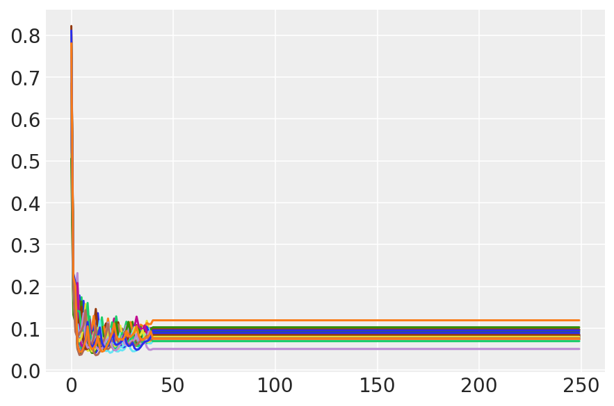
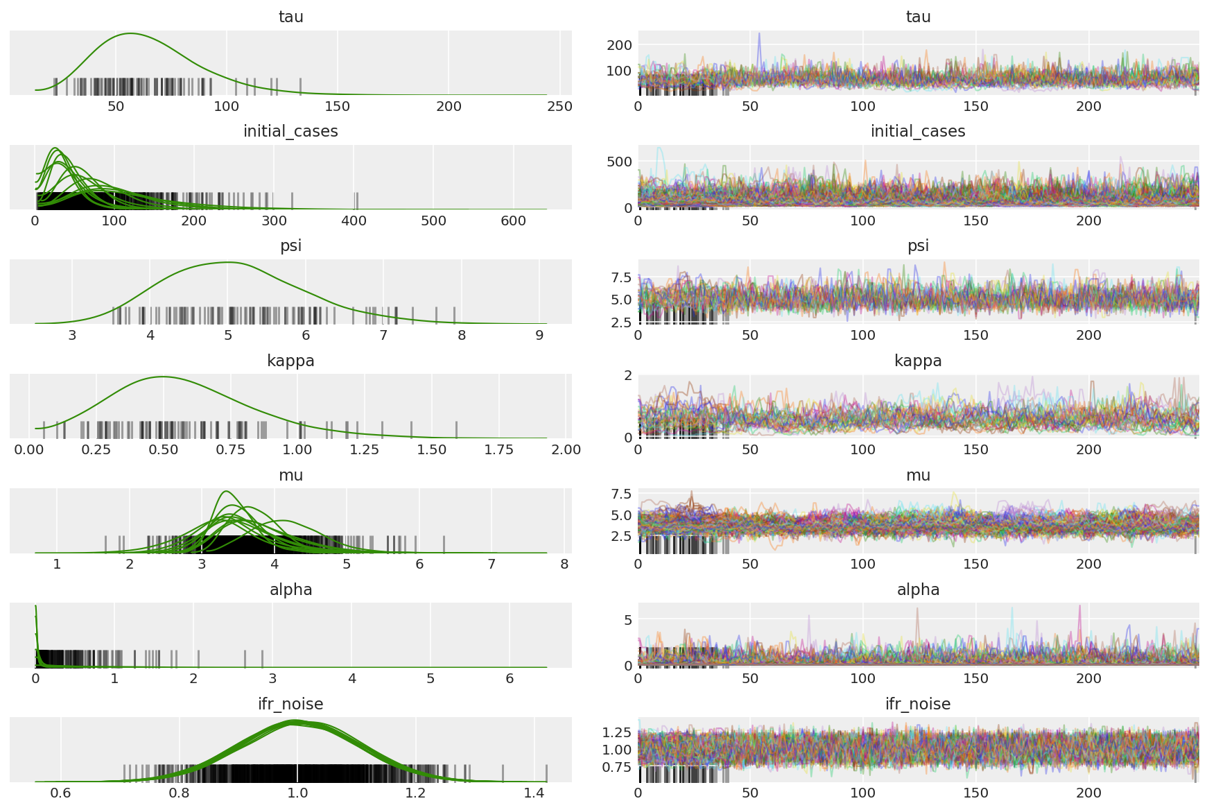
3.5 เห็นภาพตัวอย่างนำร่อง

เรากำลังมองหาโซ่ที่ติดอยู่และการบรรจบกันที่น่าจับตามอง เราสามารถทำการวินิจฉัยอย่างเป็นทางการได้ที่นี่ แต่นั่นไม่จำเป็นอย่างยิ่ง เนื่องจากเป็นเพียงการดำเนินการนำร่อง

import arviz as az
az.style.use('arviz-darkgrid')

var_name = ['tau', 'initial_cases', 'psi', 'kappa', 'mu', 'alpha', 'ifr_noise']

pilot_with_warmup = {k: np.swapaxes(v.numpy(), 1, 0)
                     for k, v in zip(var_name, pilot_samples)}

เราสังเกตความแตกต่างระหว่างการวอร์มอัพ โดยหลักแล้วเนื่องจากการปรับขนาดขั้นตอนเฉลี่ยคู่ใช้การค้นหาเชิงรุกสำหรับขนาดขั้นตอนที่เหมาะสมที่สุด เมื่อการปรับตัวปิดลง ความแตกต่างก็หายไปเช่นกัน

az_trace = az.from_dict(posterior=pilot_with_warmup,
                        sample_stats={'diverging': np.swapaxes(pilot_sampler_stat['diverging'].numpy(), 0, 1)})
az.plot_trace(az_trace, combined=True, compact=True, figsize=(12, 8));

png

plt.plot(pilot_sampler_stat['step_size'][0]);

png

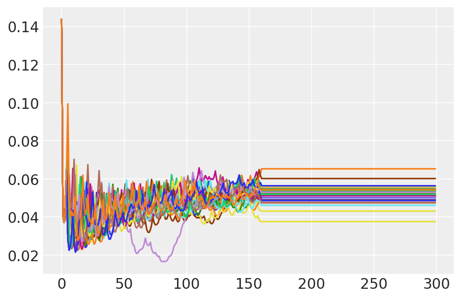
3.6 เรียกใช้ HMC

โดยหลักการแล้ว เราสามารถใช้ตัวอย่างนำร่องสำหรับการวิเคราะห์ขั้นสุดท้ายได้ (หากเรารันนานกว่าเพื่อให้ได้คอนเวอร์เจนซ์) แต่การเริ่มรัน HMC อีกครั้งจะมีประสิทธิภาพมากกว่าเล็กน้อย คราวนี้ปรับสภาพล่วงหน้าและเริ่มต้นโดยตัวอย่างนำร่อง

%%time

burnin = 50
num_steps = 200

bijectors = get_bijectors_from_samples([s[burnin:] for s in pilot_samples],
                                       unconstraining_bijectors=unconstraining_bijectors,
                                       batch_axes=(0, 1))

samples, sampler_stat = sample_hmc(
    [s[-1] for s in pilot_samples],
    [s[-1] for s in pilot_sampler_stat['step_size']],
    target_log_prob_fn,
    bijectors,
    num_steps=num_steps,
    burnin=burnin,
    num_leapfrog_steps=20)

CPU times: user 1min 26s, sys: 3.88 s, total: 1min 30s
Wall time: 1min 32s

plt.plot(sampler_stat['step_size'][0]);

png

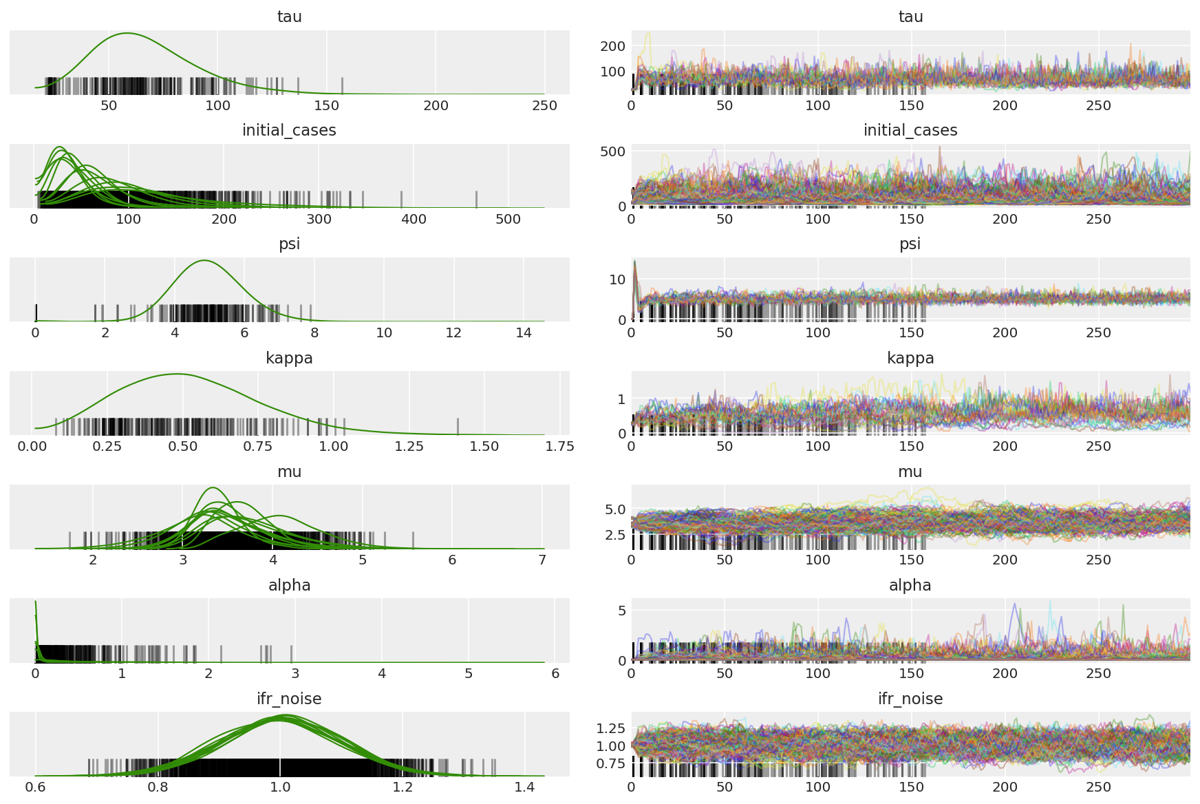
3.7 เห็นภาพตัวอย่าง

import arviz as az
az.style.use('arviz-darkgrid')

var_name = ['tau', 'initial_cases', 'psi', 'kappa', 'mu', 'alpha', 'ifr_noise']

posterior = {k: np.swapaxes(v.numpy()[burnin:], 1, 0)
             for k, v in zip(var_name, samples)}
posterior_with_warmup = {k: np.swapaxes(v.numpy(), 1, 0)
             for k, v in zip(var_name, samples)}

คำนวณบทสรุปของโซ่ เรากำลังมองหา ESS สูงและ r_hat ใกล้ 1

az.summary(posterior)

az_trace = az.from_dict(posterior=posterior_with_warmup,
                        sample_stats={'diverging': np.swapaxes(sampler_stat['diverging'].numpy(), 0, 1)})
az.plot_trace(az_trace, combined=True, compact=True, figsize=(12, 8));

png

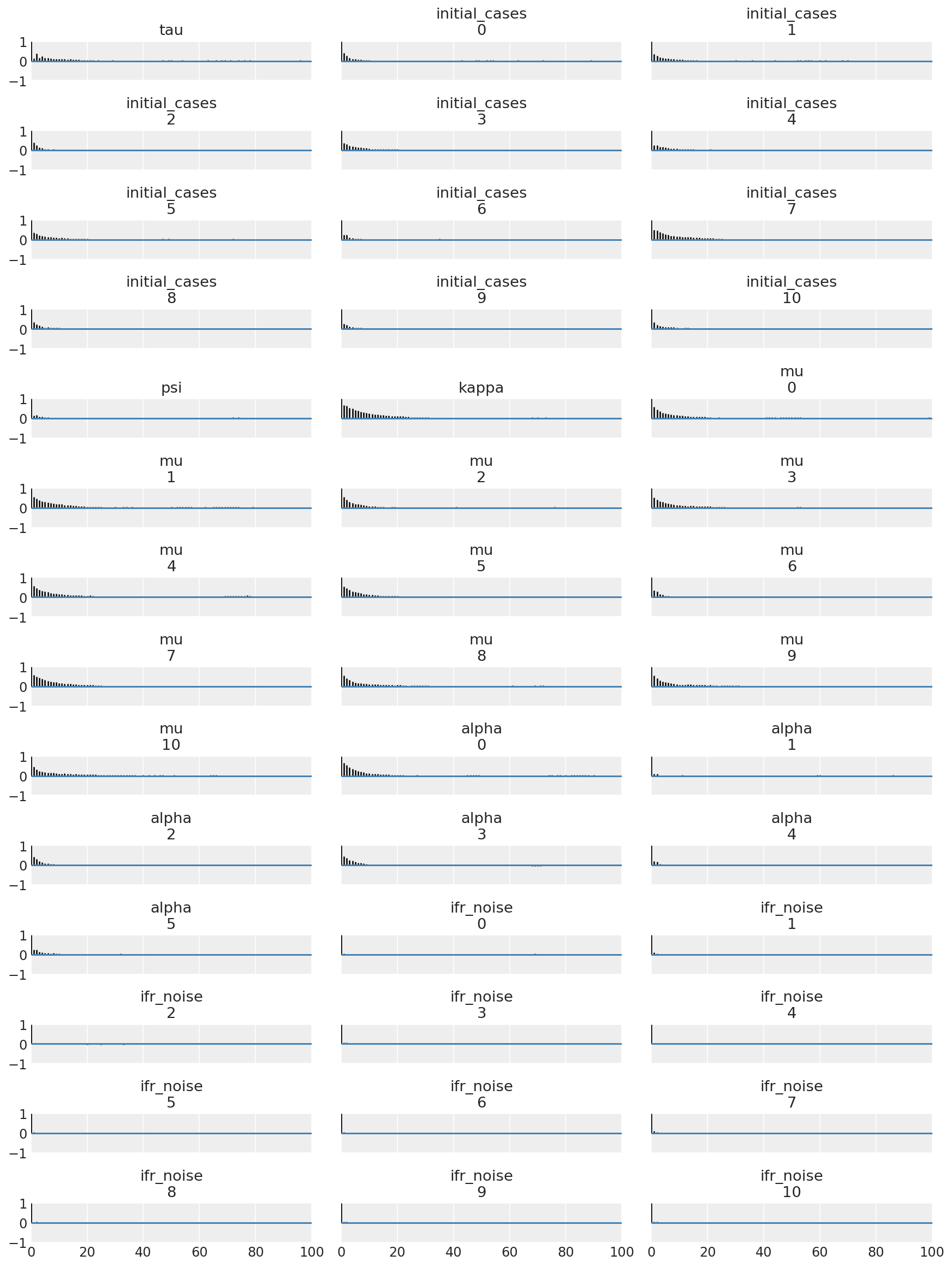
ขอแนะนำให้ดูที่ฟังก์ชันสหสัมพันธ์อัตโนมัติในทุกมิติ เรากำลังมองหาฟังก์ชันที่ลดความเร็วลงอย่างรวดเร็ว แต่ไม่มากจนเข้าไปในแง่ลบ (ซึ่งบ่งชี้ว่า HMC กระทบกระเทือน ซึ่งไม่ดีต่อการยศาสตร์และอาจทำให้เกิดอคติได้)

with az.rc_context(rc={'plot.max_subplots': None}):
  az.plot_autocorr(posterior, combined=True, figsize=(12, 16), textsize=12);

png

4 ผลลัพธ์

แปลงดังต่อไปนี้วิเคราะห์การกระจายหลังการคาดการณ์ในช่วง $R_t$ จำนวนผู้เสียชีวิตและจำนวนของการติดเชื้อที่คล้ายกับการวิเคราะห์ใน Flaxman et al, (2020).

total_num_samples = np.prod(posterior['mu'].shape[:2])

# Calculate R_t given parameter estimates.
def rt_samples_batched(mu, intervention_indicators, alpha):
  linear_prediction = tf.reduce_sum(
      intervention_indicators * alpha[..., np.newaxis, np.newaxis, :], axis=-1)
  rt_hat = mu[..., tf.newaxis] * tf.exp(-linear_prediction, name='rt')
  return rt_hat

alpha_hat = tf.convert_to_tensor(
    posterior['alpha'].reshape(total_num_samples, posterior['alpha'].shape[-1]))
mu_hat = tf.convert_to_tensor(
    posterior['mu'].reshape(total_num_samples, num_countries))
rt_hat = rt_samples_batched(mu_hat, intervention_indicators, alpha_hat)
sampled_initial_cases = posterior['initial_cases'].reshape(
    total_num_samples, num_countries)
sampled_ifr_noise = posterior['ifr_noise'].reshape(
    total_num_samples, num_countries)
psi_hat = posterior['psi'].reshape([total_num_samples])

conv_serial_interval = make_conv_serial_interval(INITIAL_DAYS, TOTAL_DAYS)
conv_fatality_rate = make_conv_fatality_rate(infection_fatality_rate, TOTAL_DAYS)
pred_hat = predict_infections(
    intervention_indicators, population_value, sampled_initial_cases, mu_hat,
    alpha_hat, conv_serial_interval, INITIAL_DAYS, TOTAL_DAYS)
expected_deaths = predict_deaths(pred_hat, sampled_ifr_noise, conv_fatality_rate)

psi_m = psi_hat[np.newaxis, ..., np.newaxis]
probs = tf.clip_by_value(expected_deaths / (expected_deaths + psi_m), 1e-9, 1.)
predicted_deaths = tfd.NegativeBinomial(
    total_count=psi_m, probs=probs).sample()

# Predict counterfactual infections/deaths in the absence of interventions
no_intervention_infections = predict_infections(
    intervention_indicators,
    population_value,
    sampled_initial_cases,
    mu_hat,
    tf.zeros_like(alpha_hat),
    conv_serial_interval,
    INITIAL_DAYS, TOTAL_DAYS)

no_intervention_expected_deaths = predict_deaths(
    no_intervention_infections, sampled_ifr_noise, conv_fatality_rate)
probs = tf.clip_by_value(
    no_intervention_expected_deaths / (no_intervention_expected_deaths + psi_m),
    1e-9, 1.)
no_intervention_predicted_deaths = tfd.NegativeBinomial(
    total_count=psi_m, probs=probs).sample()

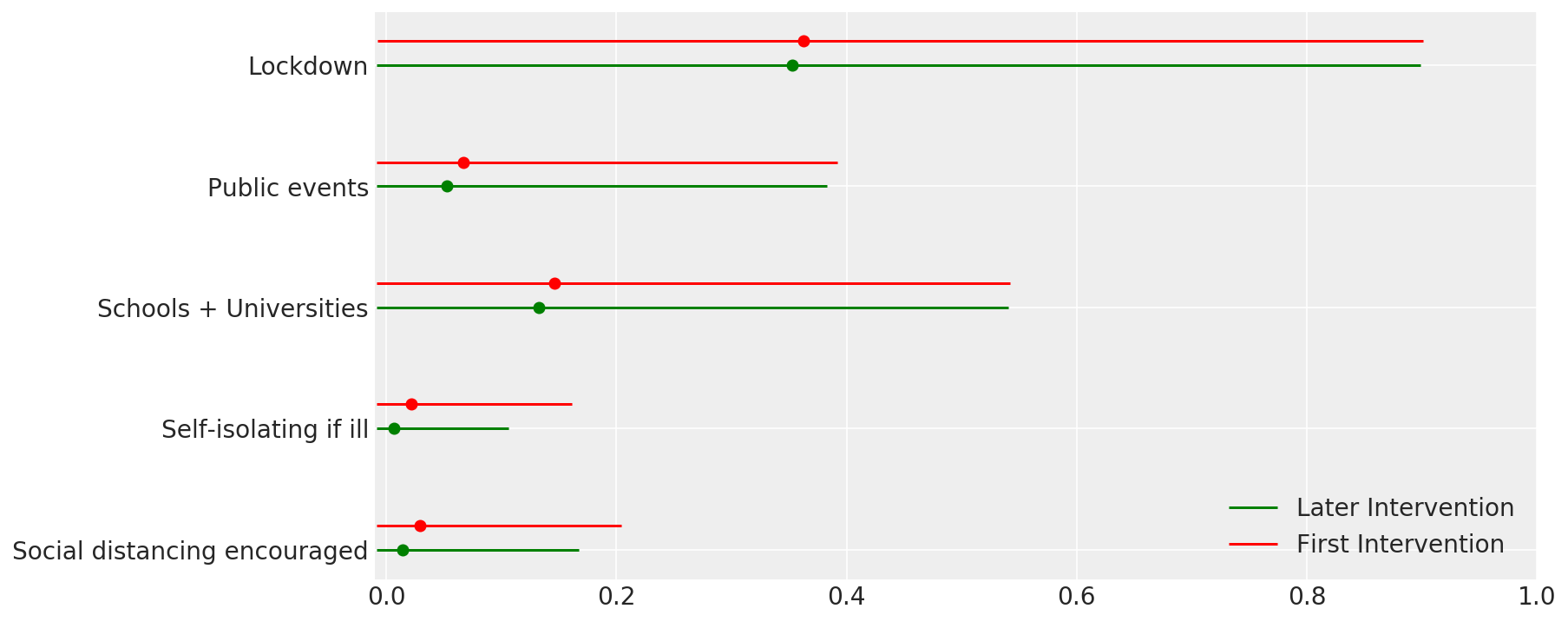
4.1 ประสิทธิผลของการแทรกแซง

คล้ายกับรูปที่ 4 ของ Flaxman et al. (2020).

def intervention_effectiveness(alpha):

  alpha_adj = 1. - np.exp(-alpha + np.log(1.05) / 6.)
  alpha_adj_first = (
      1. - np.exp(-alpha - alpha[..., -1:] + np.log(1.05) / 6.))

  fig, ax = plt.subplots(1, 1, figsize=[12, 6])
  intervention_perm = [2, 1, 3, 4, 0]
  percentile_vals = [2.5, 97.5]
  jitter = .2

  for ind in range(5):
    first_low, first_high = tfp.stats.percentile(
        alpha_adj_first[..., ind], percentile_vals)
    low, high = tfp.stats.percentile(
        alpha_adj[..., ind], percentile_vals)

    p_ind = intervention_perm[ind]
    ax.hlines(p_ind, low, high, label='Later Intervention', colors='g')
    ax.scatter(alpha_adj[..., ind].mean(), p_ind, color='g')
    ax.hlines(p_ind + jitter, first_low, first_high,
              label='First Intervention', colors='r')
    ax.scatter(alpha_adj_first[..., ind].mean(), p_ind + jitter, color='r')

    if ind == 0:
      plt.legend(loc='lower right')
  ax.set_yticks(range(5))
  ax.set_yticklabels(
      [any_intervention_list[intervention_perm.index(p)] for p in range(5)])
  ax.set_xlim([-0.01, 1.])
  r = fig.patch
  r.set_facecolor('white') 

intervention_effectiveness(alpha_hat)

png

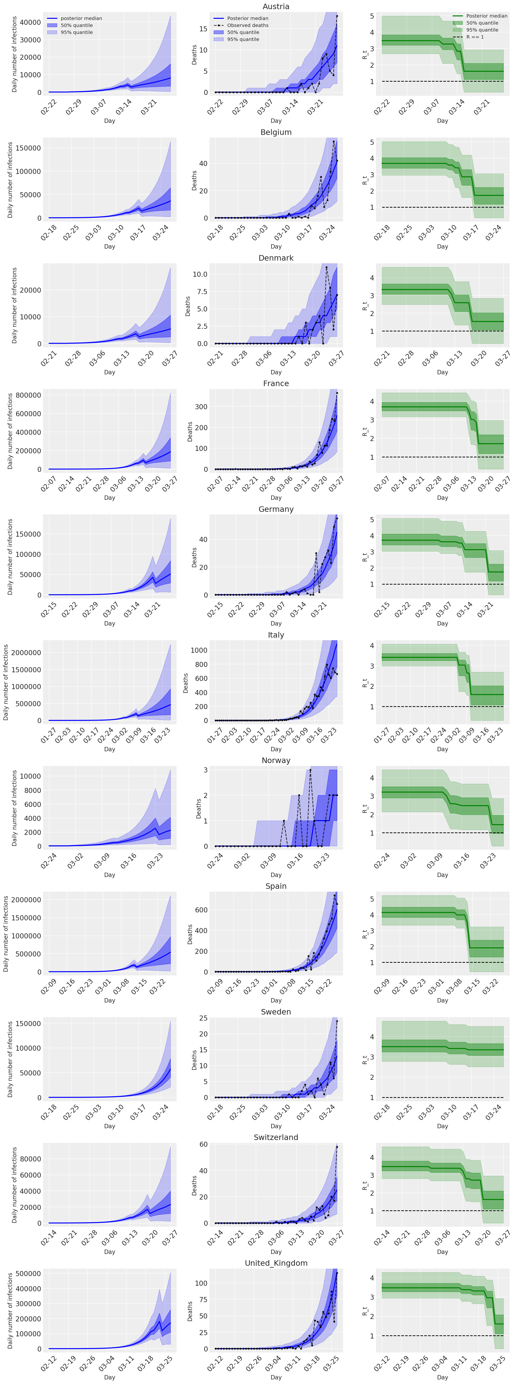
4.2 การติดเชื้อ การตาย และ R_t แยกตามประเทศ

คล้ายกับรูปที่ 2 ของ Flaxman et al. (2020).

import matplotlib.dates as mdates

plot_quantile = True
forecast_days = 0

fig, ax = plt.subplots(11, 3, figsize=(15, 40))

for ind, country in enumerate(COUNTRIES):
  num_days = (pd.to_datetime('2020-03-28') - first_days[country]).days + forecast_days
  dates = [(first_days[country] + i*pd.to_timedelta(1, 'days')).strftime('%m-%d') for i in range(num_days)]
  plot_dates = [dates[i] for i in range(0, num_days, 7)]

  # Plot daily number of infections
  infections = pred_hat[:, :, ind]
  posterior_quantile = np.percentile(infections, [2.5, 25, 50, 75, 97.5], axis=-1)
  ax[ind, 0].plot(
      dates, posterior_quantile[2, :num_days],
      color='b', label='posterior median', lw=2)
  if plot_quantile:
    ax[ind, 0].fill_between(
        dates, posterior_quantile[1, :num_days], posterior_quantile[3, :num_days],
        color='b', label='50% quantile', alpha=.4)
    ax[ind, 0].fill_between(
        dates, posterior_quantile[0, :num_days], posterior_quantile[4, :num_days],
        color='b', label='95% quantile', alpha=.2)

  ax[ind, 0].set_xticks(plot_dates)
  ax[ind, 0].xaxis.set_tick_params(rotation=45)
  ax[ind, 0].set_ylabel('Daily number of infections', fontsize='large')
  ax[ind, 0].set_xlabel('Day', fontsize='large')

  # Plot deaths
  ax[ind, 1].set_title(country)

  samples = predicted_deaths[:, :, ind]
  posterior_quantile = np.percentile(samples, [2.5, 25, 50, 75, 97.5], axis=-1)
  ax[ind, 1].plot(
      range(num_days), posterior_quantile[2, :num_days],
      color='b', label='Posterior median', lw=2)
  if plot_quantile:
    ax[ind, 1].fill_between(
        range(num_days), posterior_quantile[1, :num_days], posterior_quantile[3, :num_days],
        color='b', label='50% quantile', alpha=.4)
    ax[ind, 1].fill_between(
        range(num_days), posterior_quantile[0, :num_days], posterior_quantile[4, :num_days],
        color='b', label='95% quantile', alpha=.2)

  observed = deaths[ind, :]
  observed[observed == -1] = np.nan
  ax[ind, 1].plot(
      dates, observed[:num_days],
      '--o', color='k', markersize=3,
      label='Observed deaths', alpha=.8)
  ax[ind, 1].set_xticks(plot_dates)
  ax[ind, 1].xaxis.set_tick_params(rotation=45)
  ax[ind, 1].set_title(country)
  ax[ind, 1].set_xlabel('Day', fontsize='large')
  ax[ind, 1].set_ylabel('Deaths', fontsize='large')

  # Plot R_t
  samples = np.transpose(rt_hat[:, ind, :])
  posterior_quantile = np.percentile(samples, [2.5, 25, 50, 75, 97.5], axis=-1)
  l1 = ax[ind, 2].plot(
      dates, posterior_quantile[2, :num_days],
      color='g', label='Posterior median', lw=2)
  l2 = ax[ind, 2].fill_between(
      dates, posterior_quantile[1, :num_days], posterior_quantile[3, :num_days],
      color='g', label='50% quantile', alpha=.4)
  if plot_quantile:
    l3 = ax[ind, 2].fill_between(
        dates, posterior_quantile[0, :num_days], posterior_quantile[4, :num_days],
        color='g', label='95% quantile', alpha=.2)

  l4 = ax[ind, 2].hlines(1., dates[0], dates[-1], linestyle='--', label='R == 1')
  ax[ind, 2].set_xlabel('Day', fontsize='large')
  ax[ind, 2].set_ylabel('R_t', fontsize='large')
  ax[ind, 2].set_xticks(plot_dates)
  ax[ind, 2].xaxis.set_tick_params(rotation=45)

fontsize = 'medium'
ax[0, 0].legend(loc='upper left', fontsize=fontsize)
ax[0, 1].legend(loc='upper left', fontsize=fontsize)
ax[0, 2].legend(
  bbox_to_anchor=(1., 1.),
  loc='upper right',
  borderaxespad=0.,
  fontsize=fontsize)

plt.tight_layout();

png

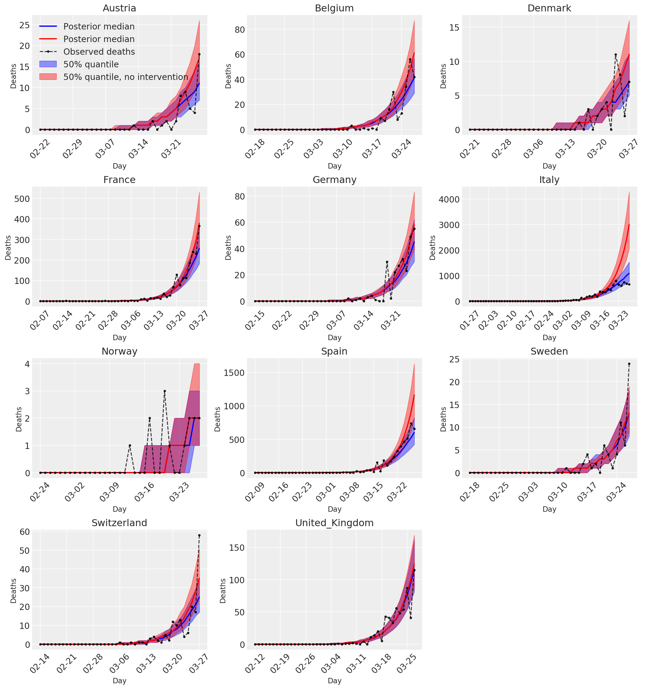
4.3 จำนวนผู้เสียชีวิตที่คาดการณ์/คาดการณ์รายวันทั้งที่มีและไม่มีการแทรกแซง

plot_quantile = True
forecast_days = 0

fig, ax = plt.subplots(4, 3, figsize=(15, 16))
ax = ax.flatten()
fig.delaxes(ax[-1])
for country_index, country in enumerate(COUNTRIES):
  num_days = (pd.to_datetime('2020-03-28') - first_days[country]).days + forecast_days
  dates = [(first_days[country] + i*pd.to_timedelta(1, 'days')).strftime('%m-%d') for i in range(num_days)]
  plot_dates = [dates[i] for i in range(0, num_days, 7)]

  ax[country_index].set_title(country)

  quantile_vals = [.025, .25, .5, .75, .975]
  samples = predicted_deaths[:, :, country_index].numpy()
  quantiles = []

  psi_m = psi_hat[np.newaxis, ..., np.newaxis]
  probs = tf.clip_by_value(expected_deaths / (expected_deaths + psi_m), 1e-9, 1.)
  predicted_deaths_dist = tfd.NegativeBinomial(
    total_count=psi_m, probs=probs)

  posterior_quantile = np.percentile(samples, [2.5, 25, 50, 75, 97.5], axis=-1)
  ax[country_index].plot(
      dates, posterior_quantile[2, :num_days],
      color='b', label='Posterior median', lw=2)
  if plot_quantile:
    ax[country_index].fill_between(
        dates, posterior_quantile[1, :num_days], posterior_quantile[3, :num_days],
        color='b', label='50% quantile', alpha=.4)

  samples_counterfact = no_intervention_predicted_deaths[:, :, country_index]
  posterior_quantile = np.percentile(samples_counterfact, [2.5, 25, 50, 75, 97.5], axis=-1)
  ax[country_index].plot(
      dates, posterior_quantile[2, :num_days],
      color='r', label='Posterior median', lw=2)
  if plot_quantile:
    ax[country_index].fill_between(
        dates, posterior_quantile[1, :num_days], posterior_quantile[3, :num_days],
        color='r', label='50% quantile, no intervention', alpha=.4)

  observed = deaths[country_index, :]
  observed[observed == -1] = np.nan
  ax[country_index].plot(
      dates, observed[:num_days],
      '--o', color='k', markersize=3,
      label='Observed deaths', alpha=.8)
  ax[country_index].set_xticks(plot_dates)
  ax[country_index].xaxis.set_tick_params(rotation=45)
  ax[country_index].set_title(country)
  ax[country_index].set_xlabel('Day', fontsize='large')
  ax[country_index].set_ylabel('Deaths', fontsize='large')
  ax[0].legend(loc='upper left')
plt.tight_layout(pad=1.0);

png