Được cấp phép theo Giấy phép MIT
# Permission is hereby granted, free of charge, to any person obtaining a copy
# of this software and associated documentation files (the "Software"), to deal
# in the Software without restriction, including without limitation the rights
# to use, copy, modify, merge, publish, distribute, sublicense, and/or sell
# copies of the Software, and to permit persons to whom the Software is
# furnished to do so, subject to the following conditions:
#
# The above copyright notice and this permission notice shall be included in all
# copies or substantial portions of the Software.
#
# THE SOFTWARE IS PROVIDED "AS IS", WITHOUT WARRANTY OF ANY KIND, EXPRESS OR
# IMPLIED, INCLUDING BUT NOT LIMITED TO THE WARRANTIES OF MERCHANTABILITY,
# FITNESS FOR A PARTICULAR PURPOSE AND NONINFRINGEMENT. IN NO EVENT SHALL THE
# AUTHORS OR COPYRIGHT HOLDERS BE LIABLE FOR ANY CLAIM, DAMAGES OR OTHER
# LIABILITY, WHETHER IN AN ACTION OF CONTRACT, TORT OR OTHERWISE, ARISING FROM,
# OUT OF OR IN CONNECTION WITH THE SOFTWARE OR THE USE OR OTHER DEALINGS IN THE
# SOFTWARE.
| | |  Xem nguồn trên GitHub Xem nguồn trên GitHub | |
Để làm chậm sự lây lan của COVID-19 vào đầu năm 2020, các nước châu Âu đã áp dụng các biện pháp can thiệp phi dược phẩm như đóng cửa các cơ sở kinh doanh không thiết yếu, cách ly các trường hợp riêng lẻ, cấm đi lại và các biện pháp khác để khuyến khích xã hội xa lánh. Các trường Imperial College COVID-19 đáp ứng Đội phân tích tính hiệu quả của các biện pháp này trong bài báo của họ "Ước tính số người nhiễm và tác động của can thiệp phi dược trên COVID-19 ở 11 quốc gia châu Âu" , sử dụng một mô hình thứ bậc Bayesian kết hợp với một cơ giới mô hình dịch tễ học.
Colab này chứa triển khai TensorFlow Probability (TFP) của phân tích đó, được tổ chức như sau:
- "Thiết lập mô hình" xác định mô hình dịch tễ học về sự lây truyền bệnh và kết quả là tử vong, phân bố trước của Bayes trên các tham số của mô hình và phân phối số ca tử vong có điều kiện dựa trên các giá trị tham số.
- "Xử lý trước dữ liệu" tải dữ liệu về thời gian và loại can thiệp ở mỗi quốc gia, số ca tử vong theo thời gian và tỷ lệ tử vong ước tính cho những người bị nhiễm bệnh.
- "Suy luận mô hình" xây dựng mô hình phân cấp Bayes và chạy Hamiltonian Monte Carlo (HMC) để lấy mẫu từ phân phối sau trên các tham số.
- "Kết quả" hiển thị các phân phối dự đoán sau cho các số lượng quan tâm như tử vong được dự báo và tử vong không thực tế trong trường hợp không có các biện pháp can thiệp.
Bài viết tìm thấy bằng chứng cho thấy các nước đã quản lý để giảm số lượng các ca nhiễm mới lây truyền qua từng người bệnh (\(R_t\)), nhưng điều đó khoảng tin cậy chứa \(R_t=1\) (giá trị trên mà dịch tiếp tục lây lan) và rằng còn quá sớm để đưa ra kết luận chắc chắn về hiệu quả của các biện pháp can thiệp. Mã Stan cho giấy nó nằm trong các tác giả Github kho, và Colab này tái bản 2 .
pip3 install -q git+git://github.com/arviz-devs/arviz.gitpip3 install -q tf-nightly tfp-nightly
Nhập khẩu
import collections
from pprint import pprint

import numpy as np
import pandas as pd

import matplotlib.pyplot as plt

%config InlineBackend.figure_format = 'retina'

import tensorflow.compat.v2 as tf
import tensorflow_probability as tfp
from tensorflow_probability.python.internal import prefer_static as ps

tf.enable_v2_behavior()

# Globally Enable XLA.
# tf.config.optimizer.set_jit(True)

try:
  physical_devices = tf.config.list_physical_devices('GPU')
  tf.config.experimental.set_memory_growth(physical_devices[0], True)
except:
  # Invalid device or cannot modify virtual devices once initialized.
  pass

tfb = tfp.bijectors
tfd = tfp.distributions

DTYPE = np.float32
1 Thiết lập mô hình
1.1 Mô hình cơ chế cho nhiễm trùng và tử vong
Mô hình lây nhiễm mô phỏng số ca lây nhiễm ở mỗi quốc gia theo thời gian. Dữ liệu đầu vào là thời gian và loại can thiệp, quy mô dân số và các trường hợp ban đầu. Các thông số kiểm soát hiệu quả của các biện pháp can thiệp và tốc độ lây truyền bệnh. Mô hình cho số người chết dự kiến áp dụng tỷ lệ tử vong cho các trường hợp nhiễm trùng được dự đoán.
Mô hình lây nhiễm thực hiện một tập hợp các lần lây nhiễm hàng ngày trước đó với sự phân bố theo khoảng cách nối tiếp (sự phân bố theo số ngày từ khi bị nhiễm bệnh đến khi lây nhiễm cho người khác). Tại mỗi bước thời gian, số ca nhiễm mới tại thời điểm \(t\), \(n_t\), được tính như sau
\ begin {method} \ sum_ {i = 0} ^ {t-1} n_i \ mu_t \ text {p} (\ text {bị lây nhiễm từ ai đó tại} i | \ text {mới bị nhiễm lúc} t) \ end { equation} nơi \(\mu_t=R_t\) và xác suất có điều kiện được lưu trữ trong conv_serial_interval , định nghĩa dưới đây.
Mô hình cho các trường hợp tử vong dự kiến thực hiện một tập hợp các trường hợp nhiễm trùng hàng ngày và sự phân bố số ngày giữa nhiễm trùng và tử vong. Đó là, trường hợp tử vong dự kiến vào ngày \(t\) được tính như sau
\ begin {equation} \ sum_ {i = 0} ^ {t-1} n_i \ text {p (chết vào ngày \(t\)| lây nhiễm vào ngày \(i\))} \ end {equation} trong đó xác suất có điều kiện được lưu trữ trong conv_fatality_rate , định nghĩa dưới đây.
from tensorflow_probability.python.internal import broadcast_util as bu

def predict_infections(
    intervention_indicators, population, initial_cases, mu, alpha_hier,
    conv_serial_interval, initial_days, total_days):
  """Predict the number of infections by forward-simulation.

  Args:
    intervention_indicators: Binary array of shape
      `[num_countries, total_days, num_interventions]`, in which `1` indicates
      the intervention is active in that country at that time and `0` indicates
      otherwise.
    population: Vector of length `num_countries`. Population of each country.
    initial_cases: Array of shape `[batch_size, num_countries]`. Number of cases
      in each country at the start of the simulation.
    mu: Array of shape `[batch_size, num_countries]`. Initial reproduction rate
      (R_0) by country.
    alpha_hier: Array of shape `[batch_size, num_interventions]` representing
      the effectiveness of interventions.
    conv_serial_interval: Array of shape
      `[total_days - initial_days, total_days]` output from
      `make_conv_serial_interval`. Convolution kernel for serial interval
      distribution.
    initial_days: Integer, number of sequential days to seed infections after
      the 10th death in a country. (N0 in the authors' Stan code.)
    total_days: Integer, number of days of observed data plus days to forecast.
      (N2 in the authors' Stan code.)
  Returns:
    predicted_infections: Array of shape
      `[total_days, batch_size, num_countries]`. (Batched) predicted number of
      infections over time and by country.
  """
  alpha = alpha_hier - tf.cast(np.log(1.05) / 6.0, DTYPE)

  # Multiply the effectiveness of each intervention in each country (alpha)
  # by the indicator variable for whether the intervention was active and sum
  # over interventions, yielding an array of shape
  # [total_days, batch_size, num_countries] that represents the total effectiveness of
  # all interventions in each country on each day (for a batch of data).
  linear_prediction = tf.einsum(
      'ijk,...k->j...i', intervention_indicators, alpha)

  # Adjust the reproduction rate per country downward, according to the
  # effectiveness of the interventions.
  rt = mu * tf.exp(-linear_prediction, name='reproduction_rate')

  # Initialize storage array for daily infections and seed it with initial
  # cases.
  daily_infections = tf.TensorArray(
      dtype=DTYPE, size=total_days, element_shape=initial_cases.shape)
  for i in range(initial_days):
    daily_infections = daily_infections.write(i, initial_cases)

  # Initialize cumulative cases.
  init_cumulative_infections = initial_cases * initial_days

  # Simulate forward for total_days days.
  cond = lambda i, *_: i < total_days
  def body(i, prev_daily_infections, prev_cumulative_infections):
    # The probability distribution over days j that someone infected on day i
    # caught the virus from someone infected on day j.
    p_infected_on_day = tf.gather(
        conv_serial_interval, i - initial_days, axis=0)

    # Multiply p_infected_on_day by the number previous infections each day and
    # by mu, and sum to obtain new infections on day i. Mu is adjusted by
    # the fraction of the population already infected, so that the population
    # size is the upper limit on the number of infections.
    prev_daily_infections_array = prev_daily_infections.stack()
    to_sum = prev_daily_infections_array * bu.left_justified_expand_dims_like(
        p_infected_on_day, prev_daily_infections_array)
    convolution = tf.reduce_sum(to_sum, axis=0)
    rt_adj = (
        (population - prev_cumulative_infections) / population
        ) * tf.gather(rt, i)
    new_infections = rt_adj * convolution

    # Update the prediction array and the cumulative number of infections.
    daily_infections = prev_daily_infections.write(i, new_infections)
    cumulative_infections = prev_cumulative_infections + new_infections
    return i + 1, daily_infections, cumulative_infections

  _, daily_infections_final, last_cumm_sum = tf.while_loop(
      cond, body,
      (initial_days, daily_infections, init_cumulative_infections),
      maximum_iterations=(total_days - initial_days))
  return daily_infections_final.stack()

def predict_deaths(predicted_infections, ifr_noise, conv_fatality_rate):
  """Expected number of reported deaths by country, by day.

  Args:
    predicted_infections: Array of shape
      `[total_days, batch_size, num_countries]` output from
      `predict_infections`.
    ifr_noise: Array of shape `[batch_size, num_countries]`. Noise in Infection
      Fatality Rate (IFR).
    conv_fatality_rate: Array of shape
      `[total_days - 1, total_days, num_countries]`. Convolutional kernel for
      calculating fatalities, output from `make_conv_fatality_rate`.
  Returns:
    predicted_deaths: Array of shape `[total_days, batch_size, num_countries]`.
      (Batched) predicted number of deaths over time and by country.
  """
  # Multiply the number of infections on day j by the probability of death
  # on day i given infection on day j, and sum over j. This yields the expected
  result_remainder = tf.einsum(
      'i...j,kij->k...j', predicted_infections, conv_fatality_rate) * ifr_noise

  # Concatenate the result with a vector of zeros so that the first day is
  # included.
  result_temp = 1e-15 * predicted_infections[:1]
  return tf.concat([result_temp, result_remainder], axis=0)
1.2 Trước giá trị tham số
Ở đây chúng tôi xác định phân phối trước chung trên các tham số mô hình. Nhiều giá trị tham số được giả định là độc lập, sao cho giá trị trước có thể được biểu thị như sau:
\(\text p(\tau, y, \psi, \kappa, \mu, \alpha) = \text p(\tau)\text p(y|\tau)\text p(\psi)\text p(\kappa)\text p(\mu|\kappa)\text p(\alpha)\text p(\epsilon)\)
trong đó:
- \(\tau\) là tham số tỷ lệ chia sẻ của phân phối mũ so với số trường hợp ban đầu ở mỗi quốc gia, \(y = y_1, ... y_{\text{num_countries} }\).
- \(\psi\) là một tham số trong việc phân phối nhị thức âm cho số trường hợp tử vong.
- \(\kappa\) là tham số quy mô chung của phân phối HalfNormal so với số sinh sản ban đầu ở mỗi nước, \(\mu = \mu_1, ..., \mu_{\text{num_countries} }\) (ghi rõ số trường hợp thêm truyền bởi mỗi người bị nhiễm).
- \(\alpha = \alpha_1, ..., \alpha_6\) là hiệu quả của mỗi trong số sáu can thiệp.
- \(\epsilon\) (gọi tắt là
ifr_noisetrong các mã, sau khi mã Stan của các tác giả) là tiếng ồn trong Nhiễm Fatality Rate (IFR).
Chúng tôi thể hiện mô hình này dưới dạng Phân phối chung TFP, một loại phân phối TFP cho phép biểu hiện các mô hình đồ họa xác suất.
def make_jd_prior(num_countries, num_interventions):
  return tfd.JointDistributionSequentialAutoBatched([
      # Rate parameter for the distribution of initial cases (tau).
      tfd.Exponential(rate=tf.cast(0.03, DTYPE)),

      # Initial cases for each country.
      lambda tau: tfd.Sample(
          tfd.Exponential(rate=tf.cast(1, DTYPE) / tau),
          sample_shape=num_countries),

      # Parameter in Negative Binomial model for deaths (psi).
      tfd.HalfNormal(scale=tf.cast(5, DTYPE)),

      # Parameter in the distribution over the initial reproduction number, R_0
      # (kappa).
      tfd.HalfNormal(scale=tf.cast(0.5, DTYPE)),

      # Initial reproduction number, R_0, for each country (mu).
      lambda kappa: tfd.Sample(
          tfd.TruncatedNormal(loc=3.28, scale=kappa, low=1e-5, high=1e5),
          sample_shape=num_countries),

      # Impact of interventions (alpha; shared for all countries).
      tfd.Sample(
          tfd.Gamma(tf.cast(0.1667, DTYPE), 1), sample_shape=num_interventions),

      # Multiplicative noise in Infection Fatality Rate.
      tfd.Sample(
          tfd.TruncatedNormal(
              loc=tf.cast(1., DTYPE), scale=0.1, low=1e-5, high=1e5),
              sample_shape=num_countries)
  ])
1.3 Khả năng tử vong được quan sát có điều kiện dựa trên các giá trị tham số
Các thể hiện mô hình khả năng \(p(\text{deaths} | \tau, y, \psi, \kappa, \mu, \alpha, \epsilon)\). Nó áp dụng các mô hình cho số ca nhiễm trùng và số ca tử vong dự kiến có điều kiện dựa trên các tham số và giả định số ca tử vong thực sự tuân theo phân phối Nhị thức Phủ định.
def make_likelihood_fn(
    intervention_indicators, population, deaths,
    infection_fatality_rate, initial_days, total_days):

  # Create a mask for the initial days of simulated data, as they are not
  # counted in the likelihood.
  observed_deaths = tf.constant(deaths.T[np.newaxis, ...], dtype=DTYPE)
  mask_temp = deaths != -1
  mask_temp[:, :START_DAYS] = False
  observed_deaths_mask = tf.constant(mask_temp.T[np.newaxis, ...])

  conv_serial_interval = make_conv_serial_interval(initial_days, total_days)
  conv_fatality_rate = make_conv_fatality_rate(
      infection_fatality_rate, total_days)

  def likelihood_fn(tau, initial_cases, psi, kappa, mu, alpha_hier, ifr_noise):
    # Run models for infections and expected deaths
    predicted_infections = predict_infections(
        intervention_indicators, population, initial_cases, mu, alpha_hier,
        conv_serial_interval, initial_days, total_days)
    e_deaths_all_countries = predict_deaths(
        predicted_infections, ifr_noise, conv_fatality_rate)

    # Construct the Negative Binomial distribution for deaths by country.
    mu_m = tf.transpose(e_deaths_all_countries, [1, 0, 2])
    psi_m = psi[..., tf.newaxis, tf.newaxis]
    probs = tf.clip_by_value(mu_m / (mu_m + psi_m), 1e-9, 1.)
    likelihood_elementwise = tfd.NegativeBinomial(
        total_count=psi_m, probs=probs).log_prob(observed_deaths)
    return tf.reduce_sum(
        tf.where(observed_deaths_mask,
                likelihood_elementwise,
                tf.zeros_like(likelihood_elementwise)),
        axis=[-2, -1])

  return likelihood_fn
1.4 Xác suất tử vong do nhiễm trùng
Phần này tính toán sự phân bố tử vong vào những ngày sau khi nhiễm bệnh. Nó giả định thời gian từ khi nhiễm bệnh đến khi chết là tổng của hai đại lượng biến thể Gamma, đại diện cho thời gian từ khi nhiễm bệnh đến khi bệnh khởi phát và thời gian từ lúc khởi phát đến khi tử vong. Sự phân bố thời gian đưa ra cái chết được kết hợp với nhiễm tử vong Tỷ lệ dữ liệu từ Verity et al. (2020) để tính xác suất của sự chết vào những ngày sau nhiễm trùng.
def daily_fatality_probability(infection_fatality_rate, total_days):
  """Computes the probability of death `d` days after infection."""

  # Convert from alternative Gamma parametrization and construct distributions
  # for number of days from infection to onset and onset to death.
  concentration1 = tf.cast((1. / 0.86)**2, DTYPE)
  rate1 = concentration1 / 5.1
  concentration2 = tf.cast((1. / 0.45)**2, DTYPE)
  rate2 = concentration2 / 18.8
  infection_to_onset = tfd.Gamma(concentration=concentration1, rate=rate1)
  onset_to_death = tfd.Gamma(concentration=concentration2, rate=rate2)

  # Create empirical distribution for number of days from infection to death.
  inf_to_death_dist = tfd.Empirical(
      infection_to_onset.sample([5e6]) + onset_to_death.sample([5e6]))

  # Subtract the CDF value at day i from the value at day i + 1 to compute the
  # probability of death on day i given infection on day 0, and given that
  # death (not recovery) is the outcome.
  times = np.arange(total_days + 1., dtype=DTYPE) + 0.5
  cdf = inf_to_death_dist.cdf(times).numpy()
  f_before_ifr = cdf[1:] - cdf[:-1]
  # Explicitly set the zeroth value to the empirical cdf at time 1.5, to include
  # the mass between time 0 and time .5.
  f_before_ifr[0] = cdf[1]

  # Multiply the daily fatality rates conditional on infection and eventual
  # death (f_before_ifr) by the infection fatality rates (probability of death
  # given intection) to obtain the probability of death on day i conditional
  # on infection on day 0.
  return infection_fatality_rate[..., np.newaxis] * f_before_ifr

def make_conv_fatality_rate(infection_fatality_rate, total_days):
  """Computes the probability of death on day `i` given infection on day `j`."""
  p_fatal_all_countries = daily_fatality_probability(
      infection_fatality_rate, total_days)

  # Use the probability of death d days after infection in each country
  # to build an array of shape [total_days - 1, total_days, num_countries],
  # where the element [i, j, c] is the probability of death on day i+1 given
  # infection on day j in country c.
  conv_fatality_rate = np.zeros(
      [total_days - 1, total_days, p_fatal_all_countries.shape[0]])
  for n in range(1, total_days):
    conv_fatality_rate[n - 1, 0:n, :] = (
        p_fatal_all_countries[:, n - 1::-1]).T
  return tf.constant(conv_fatality_rate, dtype=DTYPE)
1,5 Khoảng thời gian nối tiếp
Khoảng thời gian nối tiếp là khoảng thời gian giữa các trường hợp liên tiếp trong một chuỗi truyền bệnh và được giả định là Gamma phân bố. Chúng tôi sử dụng phân phối khoảng nối tiếp để tính xác suất mà một người bị nhiễm vào ngày \(i\) đã nhiễm bệnh từ một người trước đây bị nhiễm vào ngày \(j\) (các conv_serial_interval lập luận để predict_infections ).
def make_conv_serial_interval(initial_days, total_days):
  """Construct the convolutional kernel for infection timing."""

  g = tfd.Gamma(tf.cast(1. / (0.62**2), DTYPE), 1./(6.5*0.62**2))
  g_cdf = g.cdf(np.arange(total_days, dtype=DTYPE))

  # Approximate the probability mass function for the number of days between
  # successive infections.
  serial_interval = g_cdf[1:] - g_cdf[:-1]

  # `conv_serial_interval` is an array of shape
  # [total_days - initial_days, total_days] in which entry [i, j] contains the
  # probability that an individual infected on day i + initial_days caught the
  # virus from someone infected on day j.
  conv_serial_interval = np.zeros([total_days - initial_days, total_days])
  for n in range(initial_days, total_days):
    conv_serial_interval[n - initial_days, 0:n] = serial_interval[n - 1::-1]
  return tf.constant(conv_serial_interval, dtype=DTYPE)
2 Tiền xử lý dữ liệu
COUNTRIES = [
    'Austria',
    'Belgium',
    'Denmark',
    'France',
    'Germany',
    'Italy',
    'Norway',
    'Spain',
    'Sweden',
    'Switzerland',
    'United_Kingdom'
]
2.1 Tìm nạp và xử lý trước dữ liệu can thiệp
raw_interventions = pd.read_csv(
    'https://raw.githubusercontent.com/ImperialCollegeLondon/covid19model/master/data/interventions.csv')

raw_interventions['Date effective'] = pd.to_datetime(
    raw_interventions['Date effective'], dayfirst=True)
interventions = raw_interventions.pivot(index='Country', columns='Type', values='Date effective')

# If any interventions happened after the lockdown, use the date of the lockdown.
for col in interventions.columns:
  idx = interventions[col] > interventions['Lockdown']
  interventions.loc[idx, col] = interventions[idx]['Lockdown']

num_countries = len(COUNTRIES)
2.2 Tìm nạp dữ liệu trường hợp / tử vong và tham gia các biện pháp can thiệp
# Load the case data
data = pd.read_csv('https://raw.githubusercontent.com/ImperialCollegeLondon/covid19model/master/data/COVID-19-up-to-date.csv')
# You can also use the dataset directly from european cdc (where the ICL model fetch their data from)
# data = pd.read_csv('https://opendata.ecdc.europa.eu/covid19/casedistribution/csv')

data['country'] = data['countriesAndTerritories']
data = data[['dateRep', 'cases', 'deaths', 'country']]
data = data[data['country'].isin(COUNTRIES)]
data['dateRep'] = pd.to_datetime(data['dateRep'], format='%d/%m/%Y')

# Add 0/1 features for whether or not each intevention was in place.
data = data.join(interventions, on='country', how='outer')
for col in interventions.columns:
  data[col] = (data['dateRep'] >= data[col]).astype(int)

# Add "any_intevention" 0/1 feature.
any_intervention_list = ['Schools + Universities',
                         'Self-isolating if ill',
                         'Public events',
                         'Lockdown',
                         'Social distancing encouraged']
data['any_intervention'] = (
    data[any_intervention_list].apply(np.sum, 'columns') > 0).astype(int)

# Index by country and date.
data = data.sort_values(by=['country', 'dateRep'])
data = data.set_index(['country', 'dateRep'])
2.3 Tìm nạp và xử lý Tỷ lệ tử vong do nhiễm bệnh và dữ liệu dân số
infected_fatality_ratio = pd.read_csv(
    'https://raw.githubusercontent.com/ImperialCollegeLondon/covid19model/master/data/popt_ifr.csv')

infected_fatality_ratio = infected_fatality_ratio.replace(to_replace='United Kingdom', value='United_Kingdom')
infected_fatality_ratio['Country'] = infected_fatality_ratio.iloc[:, 1]
infected_fatality_ratio = infected_fatality_ratio[infected_fatality_ratio['Country'].isin(COUNTRIES)]
infected_fatality_ratio = infected_fatality_ratio[
  ['Country', 'popt', 'ifr']].set_index('Country')
infected_fatality_ratio = infected_fatality_ratio.sort_index()
infection_fatality_rate = infected_fatality_ratio['ifr'].to_numpy()
population_value = infected_fatality_ratio['popt'].to_numpy()
2.4 Xử lý trước dữ liệu theo quốc gia cụ thể
# Model up to 75 days of data for each country, starting 30 days before the
# tenth cumulative death.
START_DAYS = 30
MAX_DAYS = 102
COVARIATE_COLUMNS = any_intervention_list + ['any_intervention']

# Initialize an array for number of deaths.
deaths = -np.ones((num_countries, MAX_DAYS), dtype=DTYPE)

# Assuming every intervention is still inplace in the unobserved future
num_interventions = len(COVARIATE_COLUMNS)
intervention_indicators = np.ones((num_countries, MAX_DAYS, num_interventions))

first_days = {}
for i, c in enumerate(COUNTRIES):
  c_data = data.loc[c]

  # Include data only after 10th death in a country.
  mask = c_data['deaths'].cumsum() >= 10

  # Get the date that the epidemic starts in a country.
  first_day = c_data.index[mask][0] - pd.to_timedelta(START_DAYS, 'days')
  c_data = c_data.truncate(before=first_day)

  # Truncate the data after 28 March 2020 for comparison with Flaxman et al.
  c_data = c_data.truncate(after='2020-03-28')

  c_data = c_data.iloc[:MAX_DAYS]
  days_of_data = c_data.shape[0]
  deaths[i, :days_of_data] = c_data['deaths']
  intervention_indicators[i, :days_of_data] = c_data[
    COVARIATE_COLUMNS].to_numpy()
  first_days[c] = first_day

# Number of sequential days to seed infections after the 10th death in a
# country. (N0 in authors' Stan code.)
INITIAL_DAYS = 6

# Number of days of observed data plus days to forecast. (N2 in authors' Stan
# code.)
TOTAL_DAYS = deaths.shape[1]
3 Mô hình suy luận
Flaxman và cộng sự. (2020) sử dụng Stan đến mẫu từ sau tham số với Hamilton Monte Carlo (HMC) và No-U-Rẽ Sampler (NUTS).
Ở đây, chúng tôi áp dụng HMC với thích ứng kích thước bước trung bình kép. Chúng tôi sử dụng một đợt chạy thử nghiệm HMC để tiền điều kiện hóa và khởi tạo.
Suy luận sẽ chạy trong vài phút trên GPU.
3.1 Xây dựng trước và khả năng xảy ra cho mô hình
jd_prior = make_jd_prior(num_countries, num_interventions)
likelihood_fn = make_likelihood_fn(
    intervention_indicators, population_value, deaths,
    infection_fatality_rate, INITIAL_DAYS, TOTAL_DAYS)
3.2 Tiện ích
def get_bijectors_from_samples(samples, unconstraining_bijectors, batch_axes):
  """Fit bijectors to the samples of a distribution.

  This fits a diagonal covariance multivariate Gaussian transformed by the
  `unconstraining_bijectors` to the provided samples. The resultant
  transformation can be used to precondition MCMC and other inference methods.
  """
  state_std = [
      tf.math.reduce_std(bij.inverse(x), axis=batch_axes)
      for x, bij in zip(samples, unconstraining_bijectors)
  ]
  state_mu = [
      tf.math.reduce_mean(bij.inverse(x), axis=batch_axes)
      for x, bij in zip(samples, unconstraining_bijectors)
  ]
  return [tfb.Chain([cb, tfb.Shift(sh), tfb.Scale(sc)])
          for cb, sh, sc in zip(unconstraining_bijectors, state_mu, state_std)]

def generate_init_state_and_bijectors_from_prior(nchain, unconstraining_bijectors):
  """Creates an initial MCMC state, and bijectors from the prior."""
  prior_samples = jd_prior.sample(4096)

  bijectors = get_bijectors_from_samples(
      prior_samples, unconstraining_bijectors, batch_axes=0)

  init_state = [
    bij(tf.zeros([nchain] + list(s), DTYPE))
    for s, bij in zip(jd_prior.event_shape, bijectors)
  ]

  return init_state, bijectors
@tf.function(autograph=False, experimental_compile=True)
def sample_hmc(
    init_state,
    step_size,
    target_log_prob_fn,
    unconstraining_bijectors,
    num_steps=500,
    burnin=50,
    num_leapfrog_steps=10):

    def trace_fn(_, pkr):
        return {
            'target_log_prob': pkr.inner_results.inner_results.accepted_results.target_log_prob,
            'diverging': ~(pkr.inner_results.inner_results.log_accept_ratio > -1000.),
            'is_accepted': pkr.inner_results.inner_results.is_accepted,
            'step_size': [tf.exp(s) for s in pkr.log_averaging_step],
        }

    hmc = tfp.mcmc.HamiltonianMonteCarlo(
        target_log_prob_fn,
        step_size=step_size,
        num_leapfrog_steps=num_leapfrog_steps)

    hmc = tfp.mcmc.TransformedTransitionKernel(
        inner_kernel=hmc,
        bijector=unconstraining_bijectors)

    hmc = tfp.mcmc.DualAveragingStepSizeAdaptation(
        hmc,
        num_adaptation_steps=int(burnin * 0.8),
        target_accept_prob=0.8,
        decay_rate=0.5)

    # Sampling from the chain.
    return tfp.mcmc.sample_chain(
        num_results=burnin + num_steps,
        current_state=init_state,
        kernel=hmc,
        trace_fn=trace_fn)
3.3 Xác định bijector không gian sự kiện
HMC là hiệu quả nhất khi lấy mẫu từ một phân phối Gaussian đa biến đẳng hướng ( Mangoubi & Smith (2017) ), vì vậy bước đầu tiên là điều kiện tiên quyết mật độ mục tiêu để nhìn càng nhiều như thế càng tốt.
Đầu tiên và quan trọng nhất, chúng tôi chuyển đổi các biến bị ràng buộc (ví dụ: không âm) thành một không gian không bị giới hạn, mà HMC yêu cầu. Ngoài ra, chúng tôi sử dụng bijector SinhArcsinh để điều khiển độ nặng của các đuôi của mật độ mục tiêu đã biến đổi; chúng tôi muốn những để rơi ra khoảng như \(e^{-x^2}\).
unconstraining_bijectors = [
    tfb.Chain([tfb.Scale(tf.constant(1 / 0.03, DTYPE)), tfb.Softplus(),
                tfb.SinhArcsinh(tailweight=tf.constant(1.85, DTYPE))]), # tau
    tfb.Chain([tfb.Scale(tf.constant(1 / 0.03, DTYPE)), tfb.Softplus(),
                tfb.SinhArcsinh(tailweight=tf.constant(1.85, DTYPE))]), # initial_cases
    tfb.Softplus(), # psi
    tfb.Softplus(), # kappa
    tfb.Softplus(), # mu
    tfb.Chain([tfb.Scale(tf.constant(0.4, DTYPE)), tfb.Softplus(),
                tfb.SinhArcsinh(skewness=tf.constant(-0.2, DTYPE), tailweight=tf.constant(2., DTYPE))]), # alpha
    tfb.Softplus(), # ifr_noise
]
3.4 Chạy thử nghiệm HMC
Đầu tiên chúng tôi chạy HMC được điều kiện trước bởi cái trước, được khởi tạo từ số 0 trong không gian đã biến đổi. Chúng tôi không sử dụng các mẫu trước đó để khởi tạo chuỗi vì trong thực tế, những mẫu này thường dẫn đến chuỗi bị kẹt do số lượng kém.
%%time

nchain = 32

target_log_prob_fn = lambda *x: jd_prior.log_prob(*x) + likelihood_fn(*x)
init_state, bijectors = generate_init_state_and_bijectors_from_prior(nchain, unconstraining_bijectors)

# Each chain gets its own step size.
step_size = [tf.fill([nchain] + [1] * (len(s.shape) - 1), tf.constant(0.01, DTYPE)) for s in init_state]

burnin = 200
num_steps = 100

pilot_samples, pilot_sampler_stat = sample_hmc(
    init_state,
    step_size,
    target_log_prob_fn,
    bijectors,
    num_steps=num_steps,
    burnin=burnin,
    num_leapfrog_steps=10)
CPU times: user 56.8 s, sys: 2.34 s, total: 59.1 s
Wall time: 1min 1s
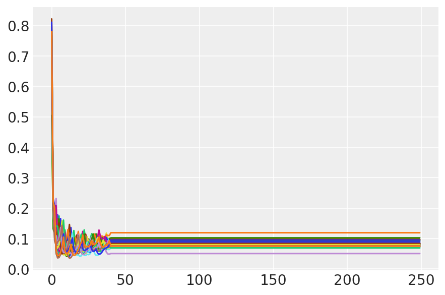
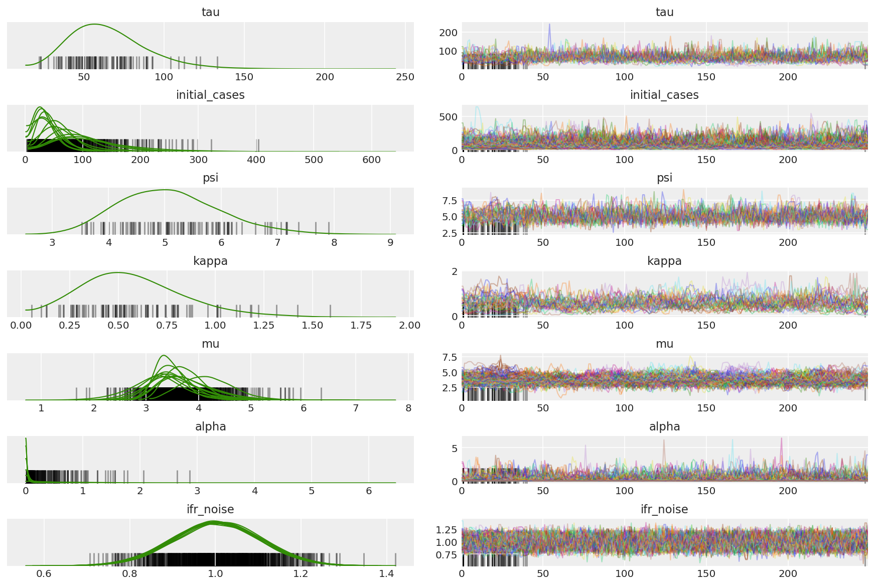
3.5 Trực quan hóa các mẫu thử nghiệm
Chúng tôi đang tìm kiếm các chuỗi bị mắc kẹt và sự hội tụ nhãn cầu. Chúng tôi có thể thực hiện chẩn đoán chính thức ở đây, nhưng điều đó không quá cần thiết vì nó chỉ là một cuộc chạy thử nghiệm.
import arviz as az
az.style.use('arviz-darkgrid')
var_name = ['tau', 'initial_cases', 'psi', 'kappa', 'mu', 'alpha', 'ifr_noise']

pilot_with_warmup = {k: np.swapaxes(v.numpy(), 1, 0)
                     for k, v in zip(var_name, pilot_samples)}
Chúng tôi quan sát thấy sự phân kỳ trong quá trình khởi động, chủ yếu là do thích ứng kích thước bước trung bình kép sử dụng tìm kiếm rất tích cực cho kích thước bước tối ưu. Một khi sự thích ứng tắt, sự phân kỳ cũng biến mất.
az_trace = az.from_dict(posterior=pilot_with_warmup,
                        sample_stats={'diverging': np.swapaxes(pilot_sampler_stat['diverging'].numpy(), 0, 1)})
az.plot_trace(az_trace, combined=True, compact=True, figsize=(12, 8));
plt.plot(pilot_sampler_stat['step_size'][0]);
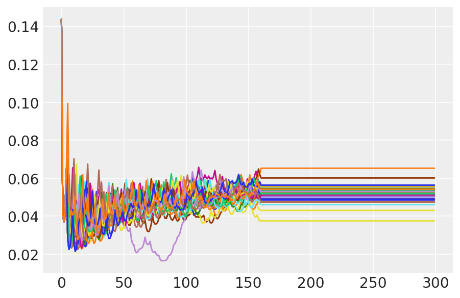
3.6 Chạy HMC
Về nguyên tắc, chúng tôi có thể sử dụng các mẫu thử nghiệm để phân tích cuối cùng (nếu chúng tôi chạy nó lâu hơn để đạt được sự hội tụ), nhưng sẽ hiệu quả hơn một chút khi bắt đầu một lần chạy HMC khác, lần này được điều chỉnh trước và khởi tạo bằng các mẫu thử nghiệm.
%%time

burnin = 50
num_steps = 200

bijectors = get_bijectors_from_samples([s[burnin:] for s in pilot_samples],
                                       unconstraining_bijectors=unconstraining_bijectors,
                                       batch_axes=(0, 1))

samples, sampler_stat = sample_hmc(
    [s[-1] for s in pilot_samples],
    [s[-1] for s in pilot_sampler_stat['step_size']],
    target_log_prob_fn,
    bijectors,
    num_steps=num_steps,
    burnin=burnin,
    num_leapfrog_steps=20)
CPU times: user 1min 26s, sys: 3.88 s, total: 1min 30s
Wall time: 1min 32s
plt.plot(sampler_stat['step_size'][0]);
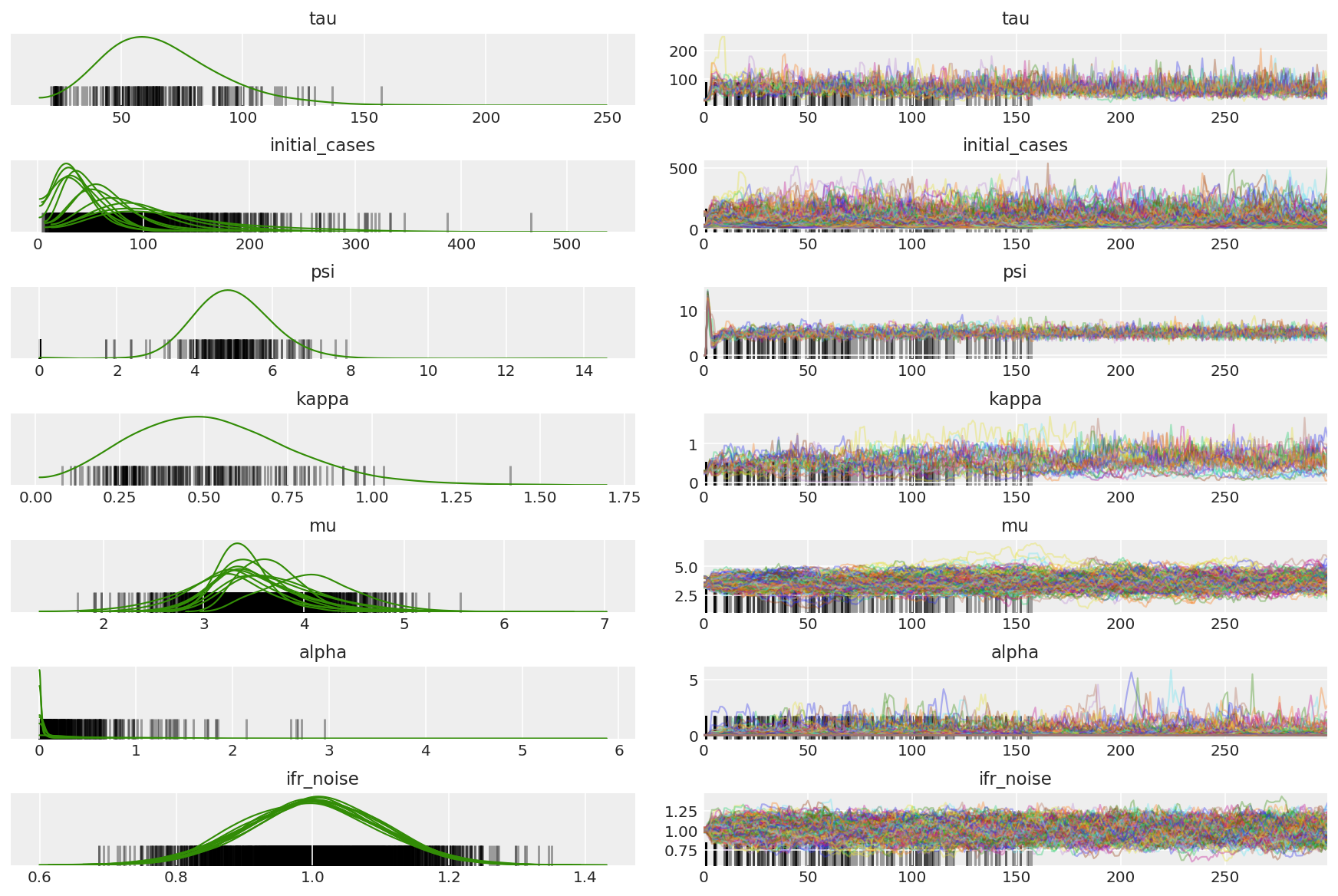
3.7 Hình dung mẫu
import arviz as az
az.style.use('arviz-darkgrid')
var_name = ['tau', 'initial_cases', 'psi', 'kappa', 'mu', 'alpha', 'ifr_noise']

posterior = {k: np.swapaxes(v.numpy()[burnin:], 1, 0)
             for k, v in zip(var_name, samples)}
posterior_with_warmup = {k: np.swapaxes(v.numpy(), 1, 0)
             for k, v in zip(var_name, samples)}
Tính toán tóm tắt của các chuỗi. Chúng tôi đang tìm kiếm ESS cao và r_hat gần bằng 1.
az.summary(posterior)
az_trace = az.from_dict(posterior=posterior_with_warmup,
                        sample_stats={'diverging': np.swapaxes(sampler_stat['diverging'].numpy(), 0, 1)})
az.plot_trace(az_trace, combined=True, compact=True, figsize=(12, 8));
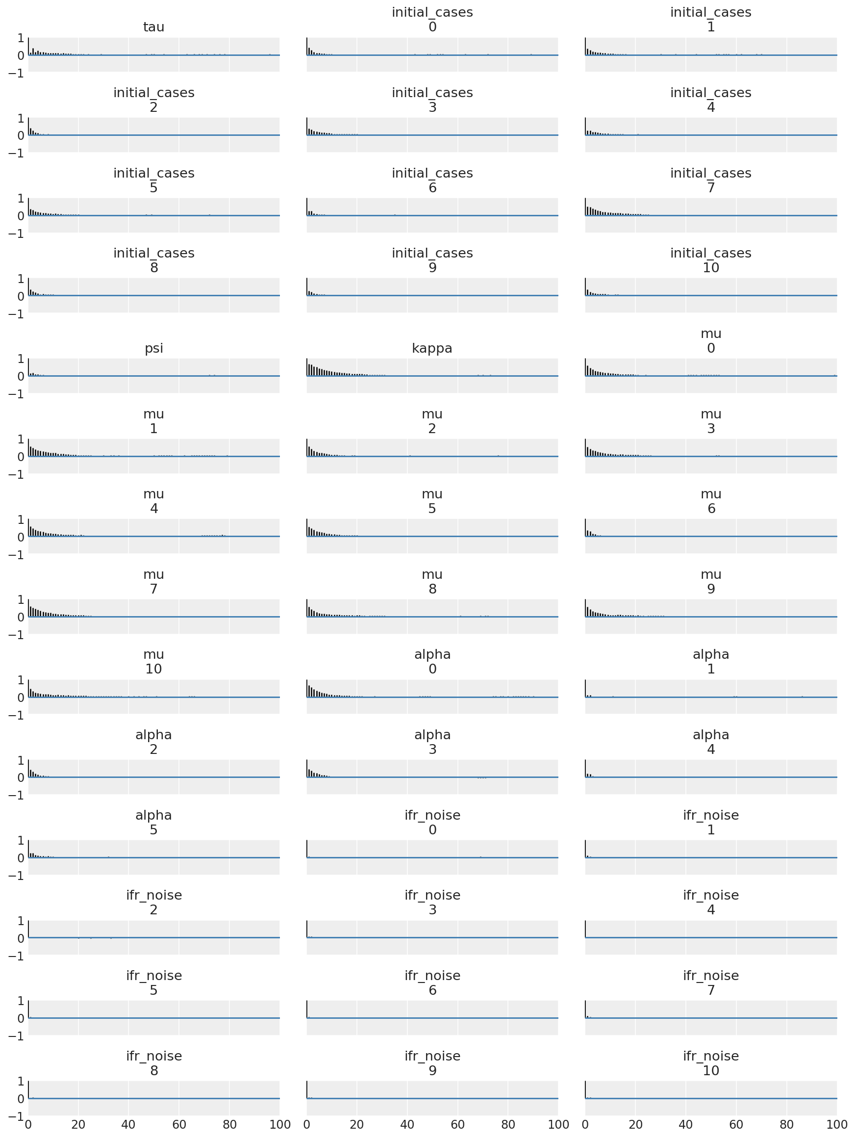
Việc xem xét các hàm tương quan tự động trên tất cả các kích thước là điều có tính hướng dẫn. Chúng tôi đang tìm kiếm các chức năng đi xuống nhanh chóng, nhưng không quá nhiều đến mức chúng đi vào âm (đó là dấu hiệu của việc HMC chạm vào một cộng hưởng, điều này không tốt cho tính ổn định và có thể gây ra sự sai lệch).
with az.rc_context(rc={'plot.max_subplots': None}):
  az.plot_autocorr(posterior, combined=True, figsize=(12, 16), textsize=12);
4 kết quả
Các lô sau phân tích sự phân bố tiên đoán hậu nghiệm qua \(R_t\), số người chết và số người nhiễm, tương tự như phân tích ở Flaxman et al. (Năm 2020).
total_num_samples = np.prod(posterior['mu'].shape[:2])

# Calculate R_t given parameter estimates.
def rt_samples_batched(mu, intervention_indicators, alpha):
  linear_prediction = tf.reduce_sum(
      intervention_indicators * alpha[..., np.newaxis, np.newaxis, :], axis=-1)
  rt_hat = mu[..., tf.newaxis] * tf.exp(-linear_prediction, name='rt')
  return rt_hat

alpha_hat = tf.convert_to_tensor(
    posterior['alpha'].reshape(total_num_samples, posterior['alpha'].shape[-1]))
mu_hat = tf.convert_to_tensor(
    posterior['mu'].reshape(total_num_samples, num_countries))
rt_hat = rt_samples_batched(mu_hat, intervention_indicators, alpha_hat)
sampled_initial_cases = posterior['initial_cases'].reshape(
    total_num_samples, num_countries)
sampled_ifr_noise = posterior['ifr_noise'].reshape(
    total_num_samples, num_countries)
psi_hat = posterior['psi'].reshape([total_num_samples])

conv_serial_interval = make_conv_serial_interval(INITIAL_DAYS, TOTAL_DAYS)
conv_fatality_rate = make_conv_fatality_rate(infection_fatality_rate, TOTAL_DAYS)
pred_hat = predict_infections(
    intervention_indicators, population_value, sampled_initial_cases, mu_hat,
    alpha_hat, conv_serial_interval, INITIAL_DAYS, TOTAL_DAYS)
expected_deaths = predict_deaths(pred_hat, sampled_ifr_noise, conv_fatality_rate)

psi_m = psi_hat[np.newaxis, ..., np.newaxis]
probs = tf.clip_by_value(expected_deaths / (expected_deaths + psi_m), 1e-9, 1.)
predicted_deaths = tfd.NegativeBinomial(
    total_count=psi_m, probs=probs).sample()
# Predict counterfactual infections/deaths in the absence of interventions
no_intervention_infections = predict_infections(
    intervention_indicators,
    population_value,
    sampled_initial_cases,
    mu_hat,
    tf.zeros_like(alpha_hat),
    conv_serial_interval,
    INITIAL_DAYS, TOTAL_DAYS)

no_intervention_expected_deaths = predict_deaths(
    no_intervention_infections, sampled_ifr_noise, conv_fatality_rate)
probs = tf.clip_by_value(
    no_intervention_expected_deaths / (no_intervention_expected_deaths + psi_m),
    1e-9, 1.)
no_intervention_predicted_deaths = tfd.NegativeBinomial(
    total_count=psi_m, probs=probs).sample()
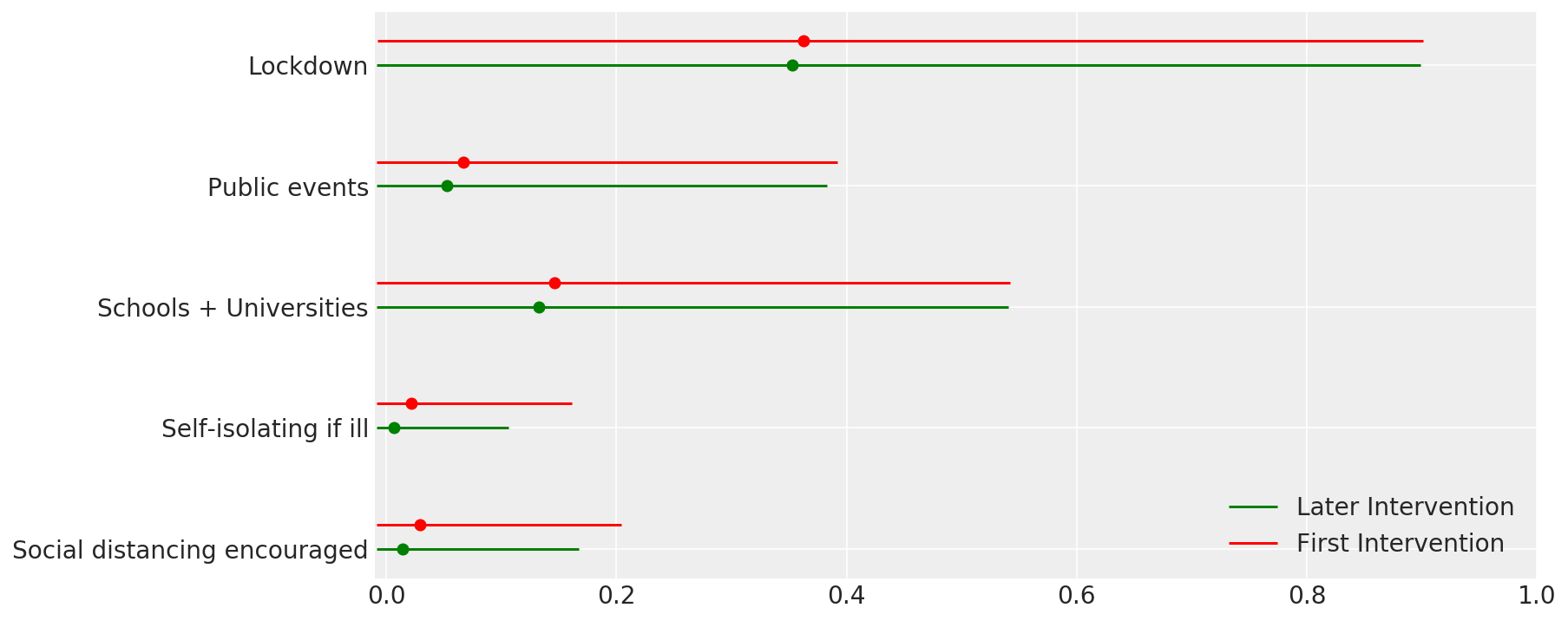
4.1 Hiệu quả của các biện pháp can thiệp
Tương tự như Hình 4 của Flaxman et al. (Năm 2020).
def intervention_effectiveness(alpha):

  alpha_adj = 1. - np.exp(-alpha + np.log(1.05) / 6.)
  alpha_adj_first = (
      1. - np.exp(-alpha - alpha[..., -1:] + np.log(1.05) / 6.))

  fig, ax = plt.subplots(1, 1, figsize=[12, 6])
  intervention_perm = [2, 1, 3, 4, 0]
  percentile_vals = [2.5, 97.5]
  jitter = .2

  for ind in range(5):
    first_low, first_high = tfp.stats.percentile(
        alpha_adj_first[..., ind], percentile_vals)
    low, high = tfp.stats.percentile(
        alpha_adj[..., ind], percentile_vals)

    p_ind = intervention_perm[ind]
    ax.hlines(p_ind, low, high, label='Later Intervention', colors='g')
    ax.scatter(alpha_adj[..., ind].mean(), p_ind, color='g')
    ax.hlines(p_ind + jitter, first_low, first_high,
              label='First Intervention', colors='r')
    ax.scatter(alpha_adj_first[..., ind].mean(), p_ind + jitter, color='r')

    if ind == 0:
      plt.legend(loc='lower right')
  ax.set_yticks(range(5))
  ax.set_yticklabels(
      [any_intervention_list[intervention_perm.index(p)] for p in range(5)])
  ax.set_xlim([-0.01, 1.])
  r = fig.patch
  r.set_facecolor('white')

intervention_effectiveness(alpha_hat)
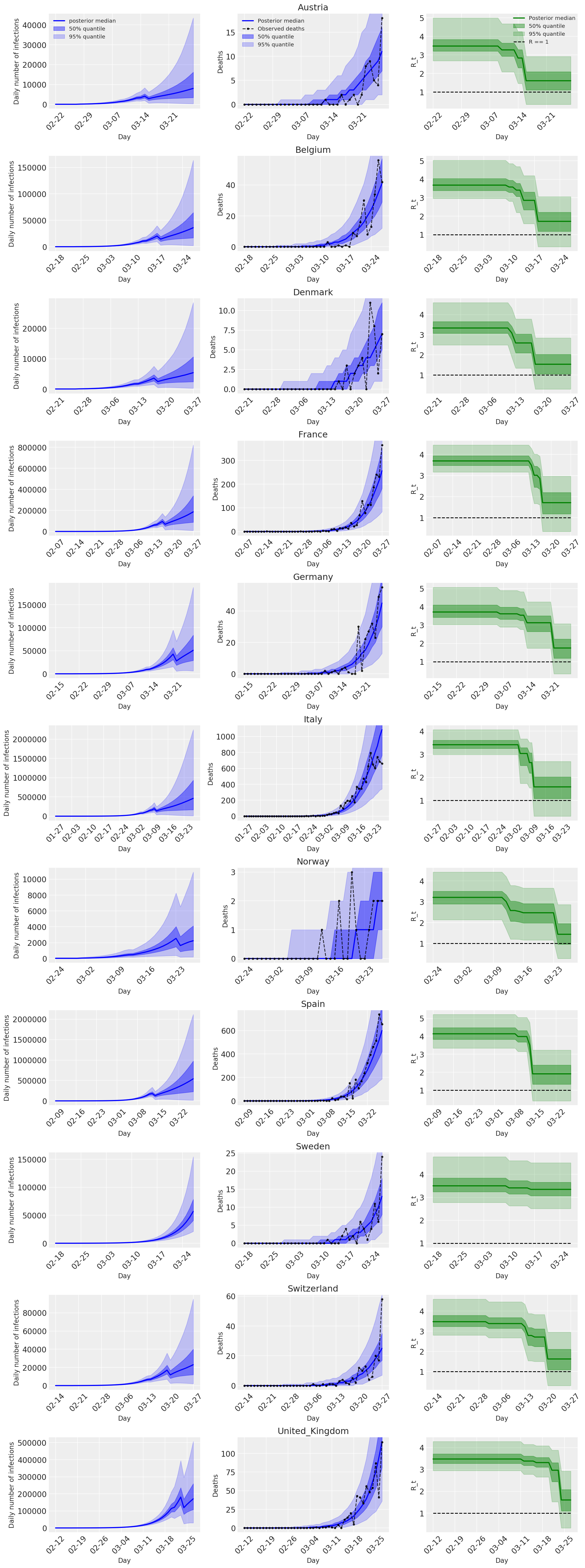
4.2 Nhiễm trùng, tử vong và R_t theo quốc gia
Tương tự như Hình 2 của Flaxman et al. (Năm 2020).
import matplotlib.dates as mdates

plot_quantile = True
forecast_days = 0

fig, ax = plt.subplots(11, 3, figsize=(15, 40))

for ind, country in enumerate(COUNTRIES):
  num_days = (pd.to_datetime('2020-03-28') - first_days[country]).days + forecast_days
  dates = [(first_days[country] + i*pd.to_timedelta(1, 'days')).strftime('%m-%d') for i in range(num_days)]
  plot_dates = [dates[i] for i in range(0, num_days, 7)]

  # Plot daily number of infections
  infections = pred_hat[:, :, ind]
  posterior_quantile = np.percentile(infections, [2.5, 25, 50, 75, 97.5], axis=-1)
  ax[ind, 0].plot(
      dates, posterior_quantile[2, :num_days],
      color='b', label='posterior median', lw=2)
  if plot_quantile:
    ax[ind, 0].fill_between(
        dates, posterior_quantile[1, :num_days], posterior_quantile[3, :num_days],
        color='b', label='50% quantile', alpha=.4)
    ax[ind, 0].fill_between(
        dates, posterior_quantile[0, :num_days], posterior_quantile[4, :num_days],
        color='b', label='95% quantile', alpha=.2)

  ax[ind, 0].set_xticks(plot_dates)
  ax[ind, 0].xaxis.set_tick_params(rotation=45)
  ax[ind, 0].set_ylabel('Daily number of infections', fontsize='large')
  ax[ind, 0].set_xlabel('Day', fontsize='large')

  # Plot deaths
  ax[ind, 1].set_title(country)

  samples = predicted_deaths[:, :, ind]
  posterior_quantile = np.percentile(samples, [2.5, 25, 50, 75, 97.5], axis=-1)
  ax[ind, 1].plot(
      range(num_days), posterior_quantile[2, :num_days],
      color='b', label='Posterior median', lw=2)
  if plot_quantile:
    ax[ind, 1].fill_between(
        range(num_days), posterior_quantile[1, :num_days], posterior_quantile[3, :num_days],
        color='b', label='50% quantile', alpha=.4)
    ax[ind, 1].fill_between(
        range(num_days), posterior_quantile[0, :num_days], posterior_quantile[4, :num_days],
        color='b', label='95% quantile', alpha=.2)

  observed = deaths[ind, :]
  observed[observed == -1] = np.nan
  ax[ind, 1].plot(
      dates, observed[:num_days],
      '--o', color='k', markersize=3,
      label='Observed deaths', alpha=.8)
  ax[ind, 1].set_xticks(plot_dates)
  ax[ind, 1].xaxis.set_tick_params(rotation=45)
  ax[ind, 1].set_title(country)
  ax[ind, 1].set_xlabel('Day', fontsize='large')
  ax[ind, 1].set_ylabel('Deaths', fontsize='large')

  # Plot R_t
  samples = np.transpose(rt_hat[:, ind, :])
  posterior_quantile = np.percentile(samples, [2.5, 25, 50, 75, 97.5], axis=-1)
  l1 = ax[ind, 2].plot(
      dates, posterior_quantile[2, :num_days],
      color='g', label='Posterior median', lw=2)
  l2 = ax[ind, 2].fill_between(
      dates, posterior_quantile[1, :num_days], posterior_quantile[3, :num_days],
      color='g', label='50% quantile', alpha=.4)
  if plot_quantile:
    l3 = ax[ind, 2].fill_between(
        dates, posterior_quantile[0, :num_days], posterior_quantile[4, :num_days],
        color='g', label='95% quantile', alpha=.2)

  l4 = ax[ind, 2].hlines(1., dates[0], dates[-1], linestyle='--', label='R == 1')
  ax[ind, 2].set_xlabel('Day', fontsize='large')
  ax[ind, 2].set_ylabel('R_t', fontsize='large')
  ax[ind, 2].set_xticks(plot_dates)
  ax[ind, 2].xaxis.set_tick_params(rotation=45)

fontsize = 'medium'
ax[0, 0].legend(loc='upper left', fontsize=fontsize)
ax[0, 1].legend(loc='upper left', fontsize=fontsize)
ax[0, 2].legend(
  bbox_to_anchor=(1., 1.),
  loc='upper right',
  borderaxespad=0.,
  fontsize=fontsize)

plt.tight_layout();
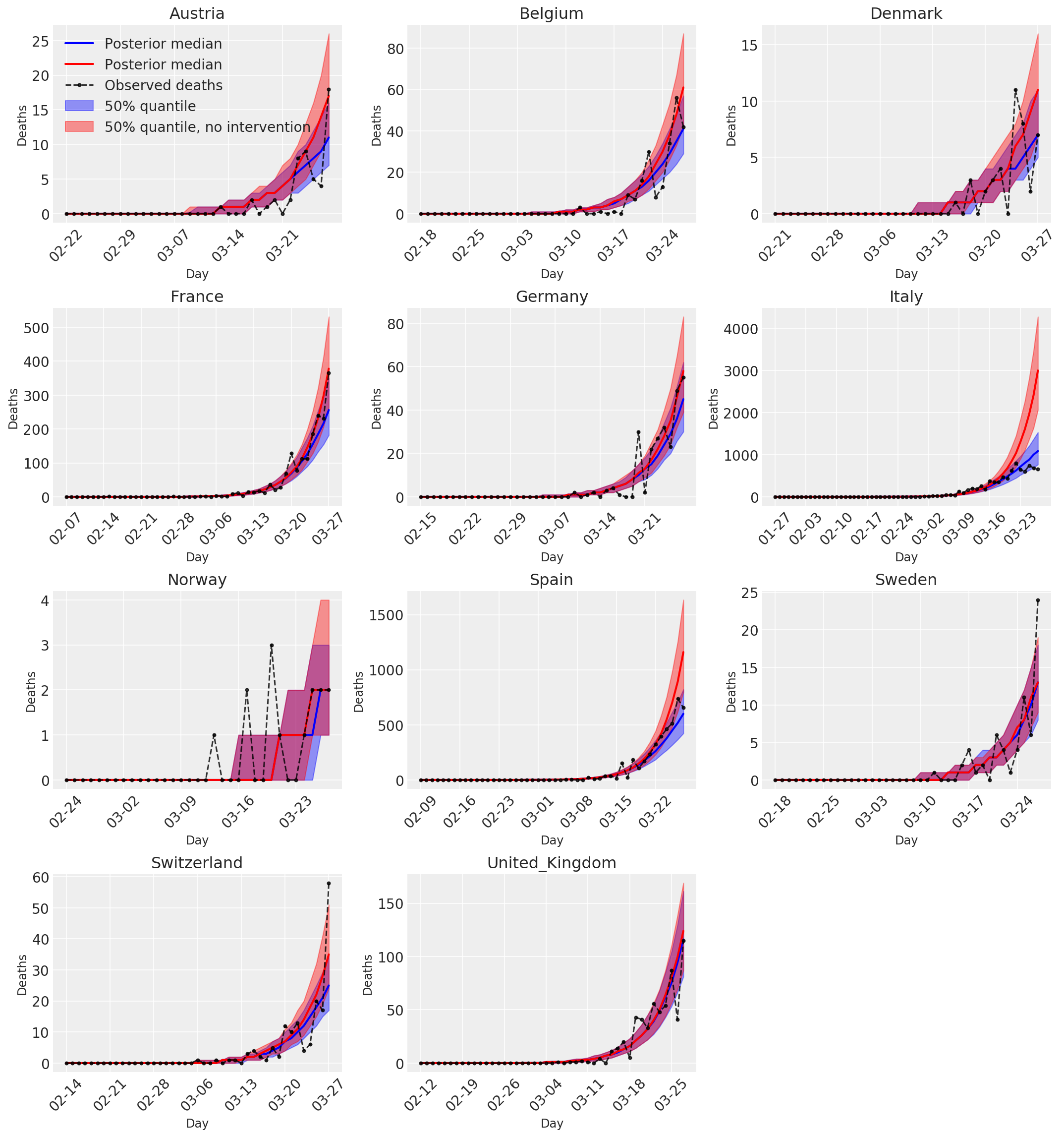
4.3 Số ca tử vong được dự đoán / dự báo hàng ngày có và không có can thiệp
plot_quantile = True
forecast_days = 0

fig, ax = plt.subplots(4, 3, figsize=(15, 16))
ax = ax.flatten()
fig.delaxes(ax[-1])
for country_index, country in enumerate(COUNTRIES):
  num_days = (pd.to_datetime('2020-03-28') - first_days[country]).days + forecast_days
  dates = [(first_days[country] + i*pd.to_timedelta(1, 'days')).strftime('%m-%d') for i in range(num_days)]
  plot_dates = [dates[i] for i in range(0, num_days, 7)]

  ax[country_index].set_title(country)

  quantile_vals = [.025, .25, .5, .75, .975]
  samples = predicted_deaths[:, :, country_index].numpy()
  quantiles = []

  psi_m = psi_hat[np.newaxis, ..., np.newaxis]
  probs = tf.clip_by_value(expected_deaths / (expected_deaths + psi_m), 1e-9, 1.)
  predicted_deaths_dist = tfd.NegativeBinomial(
    total_count=psi_m, probs=probs)

  posterior_quantile = np.percentile(samples, [2.5, 25, 50, 75, 97.5], axis=-1)
  ax[country_index].plot(
      dates, posterior_quantile[2, :num_days],
      color='b', label='Posterior median', lw=2)
  if plot_quantile:
    ax[country_index].fill_between(
        dates, posterior_quantile[1, :num_days], posterior_quantile[3, :num_days],
        color='b', label='50% quantile', alpha=.4)

  samples_counterfact = no_intervention_predicted_deaths[:, :, country_index]
  posterior_quantile = np.percentile(samples_counterfact, [2.5, 25, 50, 75, 97.5], axis=-1)
  ax[country_index].plot(
      dates, posterior_quantile[2, :num_days],
      color='r', label='Posterior median', lw=2)
  if plot_quantile:
    ax[country_index].fill_between(
        dates, posterior_quantile[1, :num_days], posterior_quantile[3, :num_days],
        color='r', label='50% quantile, no intervention', alpha=.4)

  observed = deaths[country_index, :]
  observed[observed == -1] = np.nan
  ax[country_index].plot(
      dates, observed[:num_days],
      '--o', color='k', markersize=3,
      label='Observed deaths', alpha=.8)
  ax[country_index].set_xticks(plot_dates)
  ax[country_index].xaxis.set_tick_params(rotation=45)
  ax[country_index].set_title(country)
  ax[country_index].set_xlabel('Day', fontsize='large')
  ax[country_index].set_ylabel('Deaths', fontsize='large')
  ax[0].legend(loc='upper left')
plt.tight_layout(pad=1.0);