| | |  ดูแหล่งที่มาบน GitHub ดูแหล่งที่มาบน GitHub | |
สมุดบันทึกนี้สาธิตการใช้เครื่องมือการอนุมานโดยประมาณของ TFP เพื่อรวมโมเดลการสังเกต (ที่ไม่ใช่แบบเกาส์เซียน) เมื่อทำการปรับและคาดการณ์ด้วยแบบจำลองอนุกรมเวลาเชิงโครงสร้าง (STS) ในตัวอย่างนี้ เราจะใช้แบบจำลองการสังเกตแบบปัวซองเพื่อทำงานกับข้อมูลการนับแบบไม่ต่อเนื่อง
import time
import matplotlib.pyplot as plt
import numpy as np

import tensorflow.compat.v2 as tf
import tensorflow_probability as tfp

from tensorflow_probability import bijectors as tfb
from tensorflow_probability import distributions as tfd

tf.enable_v2_behavior()
ข้อมูลสังเคราะห์
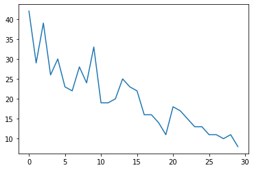
ขั้นแรกเราจะสร้างข้อมูลการนับสังเคราะห์บางส่วน:
num_timesteps = 30
observed_counts = np.round(3 + np.random.lognormal(np.log(np.linspace(
    num_timesteps, 5, num=num_timesteps)), 0.20, size=num_timesteps))
observed_counts = observed_counts.astype(np.float32)
plt.plot(observed_counts)
[<matplotlib.lines.Line2D at 0x7f940ae958d0>]
แบบอย่าง
เราจะระบุโมเดลอย่างง่ายที่มีแนวโน้มเชิงเส้นเดินสุ่ม:
def build_model(approximate_unconstrained_rates):
  trend = tfp.sts.LocalLinearTrend(
      observed_time_series=approximate_unconstrained_rates)
  return tfp.sts.Sum([trend],
                     observed_time_series=approximate_unconstrained_rates)
แทนที่จะทำงานบนอนุกรมเวลาที่สังเกตพบ โมเดลนี้จะทำงานกับชุดของพารามิเตอร์อัตราปัวซองที่ควบคุมการสังเกต
เนื่องจากอัตราปัวซองต้องเป็นค่าบวก เราจะใช้ bijector เพื่อแปลงแบบจำลอง STS ที่ประเมินมูลค่าจริงเป็นการแจกแจงเหนือค่าบวก Softplus เปลี่ยนแปลง \(y = \log(1 + \exp(x))\) เป็นทางเลือกธรรมชาติเพราะมันเป็นเกือบเชิงเส้นสำหรับค่าบวก แต่ทางเลือกอื่น ๆ เช่น Exp (ซึ่งแปลงสุ่มเดินปกติในสุ่มเดิน lognormal) ยังเป็นไปได้
positive_bijector = tfb.Softplus()  # Or tfb.Exp()

# Approximate the unconstrained Poisson rate just to set heuristic priors.
# We could avoid this by passing explicit priors on all model params.
approximate_unconstrained_rates = positive_bijector.inverse(
    tf.convert_to_tensor(observed_counts) + 0.01)
sts_model = build_model(approximate_unconstrained_rates)
ในการใช้การอนุมานโดยประมาณสำหรับโมเดลการสังเกตที่ไม่ใช่แบบเกาส์เซียน เราจะเข้ารหัสแบบจำลอง STS เป็น TFP JointDistribution ตัวแปรสุ่มในการแจกแจงร่วมนี้คือพารามิเตอร์ของแบบจำลอง STS อนุกรมเวลาของอัตราปัวซองแฝง และการนับที่สังเกตได้
def sts_with_poisson_likelihood_model():
  # Encode the parameters of the STS model as random variables.
  param_vals = []
  for param in sts_model.parameters:
    param_val = yield param.prior
    param_vals.append(param_val)

  # Use the STS model to encode the log- (or inverse-softplus)
  # rate of a Poisson.
  unconstrained_rate = yield sts_model.make_state_space_model(
      num_timesteps, param_vals)
  rate = positive_bijector.forward(unconstrained_rate[..., 0])
  observed_counts = yield tfd.Poisson(rate, name='observed_counts')

model = tfd.JointDistributionCoroutineAutoBatched(sts_with_poisson_likelihood_model)
การเตรียมการอนุมาน
เราต้องการอนุมานปริมาณที่ไม่ได้สังเกตในแบบจำลอง โดยพิจารณาจากจำนวนที่สังเกตได้ อันดับแรก เราปรับสภาพความหนาแน่นของล็อกข้อต่อบนจำนวนที่สังเกตได้
pinned_model = model.experimental_pin(observed_counts=observed_counts)
นอกจากนี้ เรายังจำเป็นต้องมีตัวส่งกำลังแบบจำกัดเพื่อให้แน่ใจว่าการอนุมานนั้นเคารพข้อจำกัดในพารามิเตอร์ของแบบจำลอง STS (เช่น มาตราส่วนต้องเป็นค่าบวก)
constraining_bijector = pinned_model.experimental_default_event_space_bijector()
การอนุมานด้วย HMC
เราจะใช้ HMC (โดยเฉพาะ NUTS) เพื่อสุ่มตัวอย่างจากส่วนหลังร่วมเหนือพารามิเตอร์แบบจำลองและอัตราแฝง
ซึ่งจะช้ากว่าการปรับรุ่น STS มาตรฐานกับ HMC อย่างมีนัยสำคัญ เนื่องจากนอกจากพารามิเตอร์ของรุ่น (จำนวนค่อนข้างน้อย) แล้ว เรายังต้องอนุมานชุดอัตรา Poisson ทั้งหมดด้วย ดังนั้นเราจะดำเนินการตามขั้นตอนที่ค่อนข้างน้อย สำหรับแอปพลิเคชันที่คุณภาพการอนุมานเป็นสิ่งสำคัญ การเพิ่มค่าเหล่านี้หรือรันหลายเชนอาจสมเหตุสมผล
การกำหนดค่าตัวอย่าง
# Allow external control of sampling to reduce test runtimes.
num_results = 500 # @param { isTemplate: true}
num_results = int(num_results)

num_burnin_steps = 100 # @param { isTemplate: true}
num_burnin_steps = int(num_burnin_steps)
ครั้งแรกที่เราระบุตัวอย่างและจากนั้นใช้ sample_chain ที่จะเรียกว่าการสุ่มตัวอย่างเคอร์เนลตัวอย่างการผลิต
sampler = tfp.mcmc.TransformedTransitionKernel(
    tfp.mcmc.NoUTurnSampler(
        target_log_prob_fn=pinned_model.unnormalized_log_prob,
        step_size=0.1),
    bijector=constraining_bijector)

adaptive_sampler = tfp.mcmc.DualAveragingStepSizeAdaptation(
    inner_kernel=sampler,
    num_adaptation_steps=int(0.8 * num_burnin_steps),
    target_accept_prob=0.75)

initial_state = constraining_bijector.forward(
    type(pinned_model.event_shape)(
        *(tf.random.normal(part_shape)
          for part_shape in constraining_bijector.inverse_event_shape(
              pinned_model.event_shape))))
# Speed up sampling by tracing with `tf.function`.
@tf.function(autograph=False, jit_compile=True)
def do_sampling():
  return tfp.mcmc.sample_chain(
      kernel=adaptive_sampler,
      current_state=initial_state,
      num_results=num_results,
      num_burnin_steps=num_burnin_steps,
      trace_fn=None)

t0 = time.time()
samples = do_sampling()
t1 = time.time()
print("Inference ran in {:.2f}s.".format(t1-t0))
Inference ran in 24.83s.
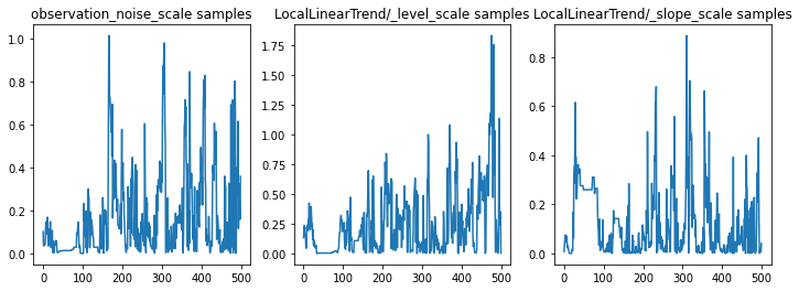
เรามีสติสัมปชัญญะ-ตรวจสอบการอนุมานได้โดยการตรวจติดตามพารามิเตอร์ ในกรณีนี้ ดูเหมือนว่าพวกเขาจะได้สำรวจคำอธิบายหลายๆ อย่างสำหรับข้อมูล ซึ่งถือว่าดี แม้ว่าตัวอย่างจำนวนมากจะมีประโยชน์ในการตัดสินว่าห่วงโซ่ผสมกันได้ดีเพียงใด
f = plt.figure(figsize=(12, 4))
for i, param in enumerate(sts_model.parameters):
  ax = f.add_subplot(1, len(sts_model.parameters), i + 1)
  ax.plot(samples[i])
  ax.set_title("{} samples".format(param.name))
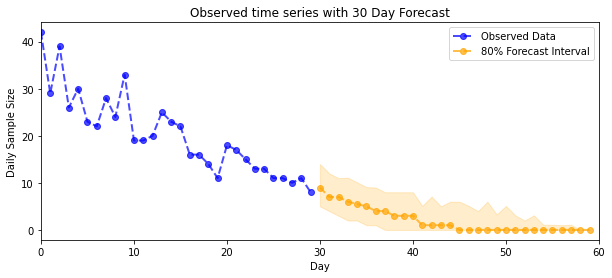
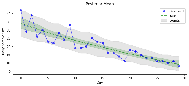
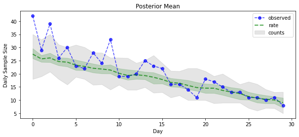
สำหรับผลตอบแทน: มาดูอัตรา Poisson ย้อนหลังกัน! นอกจากนี้ เราจะพล็อตช่วงการคาดการณ์ 80% ของจำนวนที่สังเกตได้ และสามารถตรวจสอบว่าช่วงเวลานี้ดูเหมือนจะประกอบด้วยประมาณ 80% ของการนับที่เราสังเกตจริง
param_samples = samples[:-1]
unconstrained_rate_samples = samples[-1][..., 0]
rate_samples = positive_bijector.forward(unconstrained_rate_samples)

plt.figure(figsize=(10, 4))
mean_lower, mean_upper = np.percentile(rate_samples, [10, 90], axis=0)
pred_lower, pred_upper = np.percentile(np.random.poisson(rate_samples),
                                       [10, 90], axis=0)

_ = plt.plot(observed_counts, color="blue", ls='--', marker='o', label='observed', alpha=0.7)
_ = plt.plot(np.mean(rate_samples, axis=0), label='rate', color="green", ls='dashed', lw=2, alpha=0.7)
_ = plt.fill_between(np.arange(0, 30), mean_lower, mean_upper, color='green', alpha=0.2)
_ = plt.fill_between(np.arange(0, 30), pred_lower, pred_upper, color='grey', label='counts', alpha=0.2)
plt.xlabel("Day")
plt.ylabel("Daily Sample Size")
plt.title("Posterior Mean")
plt.legend()
<matplotlib.legend.Legend at 0x7f93ffd35550>
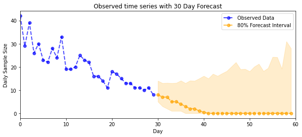
พยากรณ์
ในการคาดการณ์จำนวนที่สังเกตได้ เราจะใช้เครื่องมือ STS มาตรฐานเพื่อสร้างการกระจายการคาดการณ์เหนืออัตราแฝง (ในพื้นที่ที่ไม่มีข้อจำกัด อีกครั้งเนื่องจาก STS ได้รับการออกแบบมาเพื่อจำลองข้อมูลมูลค่าจริง) จากนั้นจึงส่งการคาดการณ์ตัวอย่างผ่านการสังเกตแบบปัวซอง แบบอย่าง:
def sample_forecasted_counts(sts_model, posterior_latent_rates,
                             posterior_params, num_steps_forecast,
                             num_sampled_forecasts):

  # Forecast the future latent unconstrained rates, given the inferred latent
  # unconstrained rates and parameters.
  unconstrained_rates_forecast_dist = tfp.sts.forecast(sts_model,
    observed_time_series=unconstrained_rate_samples,
    parameter_samples=posterior_params,
    num_steps_forecast=num_steps_forecast)

  # Transform the forecast to positive-valued Poisson rates.
  rates_forecast_dist = tfd.TransformedDistribution(
      unconstrained_rates_forecast_dist,
      positive_bijector)

  # Sample from the forecast model following the chain rule:
  # P(counts) = P(counts | latent_rates)P(latent_rates)
  sampled_latent_rates = rates_forecast_dist.sample(num_sampled_forecasts)
  sampled_forecast_counts = tfd.Poisson(rate=sampled_latent_rates).sample()

  return sampled_forecast_counts, sampled_latent_rates

forecast_samples, rate_samples = sample_forecasted_counts(
   sts_model,
   posterior_latent_rates=unconstrained_rate_samples,
   posterior_params=param_samples,
   # Days to forecast:
   num_steps_forecast=30,
   num_sampled_forecasts=100)
forecast_samples = np.squeeze(forecast_samples)
def plot_forecast_helper(data, forecast_samples, CI=90):
  """Plot the observed time series alongside the forecast."""
  plt.figure(figsize=(10, 4))
  forecast_median = np.median(forecast_samples, axis=0)

  num_steps = len(data)
  num_steps_forecast = forecast_median.shape[-1]

  plt.plot(np.arange(num_steps), data, lw=2, color='blue', linestyle='--', marker='o',
           label='Observed Data', alpha=0.7)

  forecast_steps = np.arange(num_steps, num_steps+num_steps_forecast)

  CI_interval = [(100 - CI)/2, 100 - (100 - CI)/2]
  lower, upper = np.percentile(forecast_samples, CI_interval, axis=0)

  plt.plot(forecast_steps, forecast_median, lw=2, ls='--', marker='o', color='orange',
           label=str(CI) + '% Forecast Interval', alpha=0.7)
  plt.fill_between(forecast_steps,
                   lower,
                   upper, color='orange', alpha=0.2)

  plt.xlim([0, num_steps+num_steps_forecast])
  ymin, ymax = min(np.min(forecast_samples), np.min(data)), max(np.max(forecast_samples), np.max(data))
  yrange = ymax-ymin
  plt.title("{}".format('Observed time series with ' + str(num_steps_forecast) + ' Day Forecast'))
  plt.xlabel('Day')
  plt.ylabel('Daily Sample Size')
  plt.legend()
plot_forecast_helper(observed_counts, forecast_samples, CI=80)
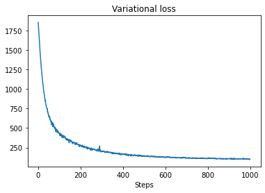
VI การอนุมาน
แปรผันอนุมานได้เป็นปัญหาเมื่ออนุมานแบบเต็มเวลาเช่นการนับจำนวนโดยประมาณของเรา (เมื่อเทียบกับเพียงพารามิเตอร์ของอนุกรมเวลาที่เป็นมาตรฐานในรุ่นเอสที) สมมติฐานมาตรฐานที่ว่าตัวแปรมีส่วนหลังที่เป็นอิสระนั้นค่อนข้างผิด เนื่องจากแต่ละขั้นตอนเวลามีความสัมพันธ์กับเพื่อนบ้าน ซึ่งอาจนำไปสู่การประเมินความไม่แน่นอนต่ำเกินไป ด้วยเหตุผลนี้ HMC อาจเป็นทางเลือกที่ดีกว่าสำหรับการอนุมานโดยประมาณในชุดข้อมูลเต็มเวลา อย่างไรก็ตาม VI อาจเร็วกว่าเล็กน้อย และอาจมีประโยชน์สำหรับการสร้างต้นแบบโมเดล หรือในกรณีที่สามารถแสดงประสิทธิภาพได้อย่างชัดเจนว่า 'ดีเพียงพอ'
เพื่อให้พอดีกับแบบจำลองของเรากับ VI เราเพียงแค่สร้างและเพิ่มประสิทธิภาพตัวแทนเสมือนหลัง:
surrogate_posterior = tfp.experimental.vi.build_factored_surrogate_posterior(
    event_shape=pinned_model.event_shape,
    bijector=constraining_bijector)
# Allow external control of optimization to reduce test runtimes.
num_variational_steps = 1000 # @param { isTemplate: true}
num_variational_steps = int(num_variational_steps)

t0 = time.time()
losses = tfp.vi.fit_surrogate_posterior(pinned_model.unnormalized_log_prob,
                                        surrogate_posterior,
                                        optimizer=tf.optimizers.Adam(0.1),
                                        num_steps=num_variational_steps)
t1 = time.time()
print("Inference ran in {:.2f}s.".format(t1-t0))
Inference ran in 11.37s.
plt.plot(losses)
plt.title("Variational loss")
_ = plt.xlabel("Steps")
posterior_samples = surrogate_posterior.sample(50)
param_samples = posterior_samples[:-1]
unconstrained_rate_samples = posterior_samples[-1][..., 0]
rate_samples = positive_bijector.forward(unconstrained_rate_samples)

plt.figure(figsize=(10, 4))
mean_lower, mean_upper = np.percentile(rate_samples, [10, 90], axis=0)
pred_lower, pred_upper = np.percentile(
    np.random.poisson(rate_samples), [10, 90], axis=0)

_ = plt.plot(observed_counts, color='blue', ls='--', marker='o',
             label='observed', alpha=0.7)
_ = plt.plot(np.mean(rate_samples, axis=0), label='rate', color='green',
             ls='dashed', lw=2, alpha=0.7)
_ = plt.fill_between(
    np.arange(0, 30), mean_lower, mean_upper, color='green', alpha=0.2)
_ = plt.fill_between(np.arange(0, 30), pred_lower, pred_upper, color='grey',
    label='counts', alpha=0.2)
plt.xlabel('Day')
plt.ylabel('Daily Sample Size')
plt.title('Posterior Mean')
plt.legend()
<matplotlib.legend.Legend at 0x7f93ff4735c0>
forecast_samples, rate_samples = sample_forecasted_counts(
   sts_model,
   posterior_latent_rates=unconstrained_rate_samples,
   posterior_params=param_samples,
   # Days to forecast:
   num_steps_forecast=30,
   num_sampled_forecasts=100)
forecast_samples = np.squeeze(forecast_samples)
plot_forecast_helper(observed_counts, forecast_samples, CI=80)