|
|
|
 在 GitHub 上查看源代码 在 GitHub 上查看源代码
|
|
本教程是使用基于 tf.estimator API的决策树来训练梯度提升模型的端到端演示。提升树(Boosted Trees)模型是回归和分类问题中最受欢迎并最有效的机器学习方法之一。这是一种融合技术,它结合了几个(10 个,100 个或者甚至 1000 个)树模型的预测值。
提升树(Boosted Trees)模型受到许多机器学习从业者的欢迎,因为它们可以通过最小化的超参数调整获得令人印象深刻的性能。
加载泰坦尼克数据集
您将使用泰坦尼克数据集,该数据集的目标是在给出性别、年龄、阶级等特征的条件下预测乘客幸存与否。
import numpy as np
import pandas as pd
from IPython.display import clear_output
from matplotlib import pyplot as plt

# 加载数据集。
dftrain = pd.read_csv('https://storage.googleapis.com/tf-datasets/titanic/train.csv')
dfeval = pd.read_csv('https://storage.googleapis.com/tf-datasets/titanic/eval.csv')
y_train = dftrain.pop('survived')
y_eval = dfeval.pop('survived')
import tensorflow as tf
tf.random.set_seed(123)
数据集由训练集和验证集组成:
dftrain与y_train是训练集——模型用来学习的数据。- 模型根据评估集,
dfeval和y_eval进行测试。
您将使用以下特征来进行训练:
| 特征名称 | 描述 |
|---|---|
| sex | 乘客的性别 |
| age | 乘客的年龄 |
| n_siblings_spouses | 船上的兄弟姐妹与伙伴 |
| parch | 船上的父母与孩子 |
| fare | 乘客所支付的票价 |
| class | 乘客在船上的舱室等级 |
| deck | 哪个甲板上的乘客 |
| embark_town | 乘客是从哪个城镇上船的 |
| alone | 是否乘客独自一人 |
探索数据
让我们首先预览一些数据,并在训练集上创建摘要统计。
dftrain.head()
dftrain.describe()
训练集和评估集分别有 627 和 264 个样本。
dftrain.shape[0], dfeval.shape[0]
(627, 264)
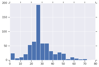
大多数乘客在 20 岁或 30 岁。
dftrain.age.hist(bins=20)
plt.show()
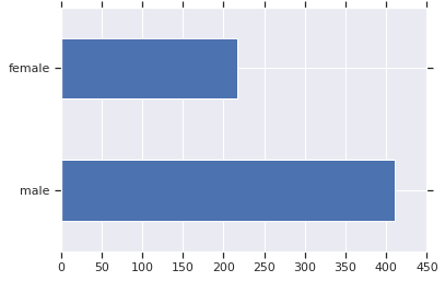
男乘客大约是女乘客的两倍。
dftrain.sex.value_counts().plot(kind='barh')
plt.show()
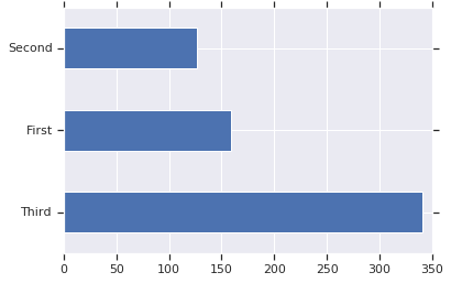
大多数乘客都在“三等”舱。
dftrain['class'].value_counts().plot(kind='barh')
plt.show()
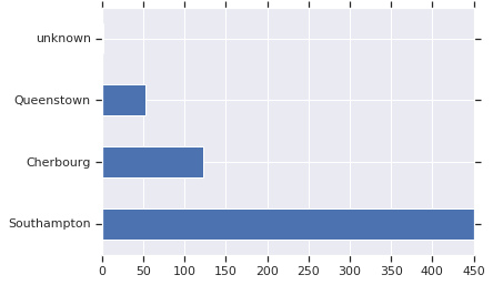
大多数乘客从南安普顿出发。
dftrain['embark_town'].value_counts().plot(kind='barh')
plt.show()
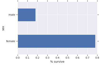
与男性相比,女性存活的几率要高得多。这显然是该模型的预测特征。
pd.concat([dftrain, y_train], axis=1).groupby('sex').survived.mean().plot(kind='barh').set_xlabel('% survive')
plt.show()
创建特征列与输入函数
梯度提升(Gradient Boosting) Estimator 可以利用数值和分类特征。特征列适用于所有的 Tensorflow estimator,其目的是定义用于建模的特征。此外,它们还提供一些特征工程功能,如独热编码(one-hot-encoding)、标准化(normalization)和桶化(bucketization)。在本教程中,CATEGORICAL_COLUMNS 中的字段从分类列转换为独热编码列(指标列):
fc = tf.feature_column
CATEGORICAL_COLUMNS = ['sex', 'n_siblings_spouses', 'parch', 'class', 'deck',
                       'embark_town', 'alone']
NUMERIC_COLUMNS = ['age', 'fare']

def one_hot_cat_column(feature_name, vocab):
  return tf.feature_column.indicator_column(
      tf.feature_column.categorical_column_with_vocabulary_list(feature_name,
                                                 vocab))
feature_columns = []
for feature_name in CATEGORICAL_COLUMNS:
  # Need to one-hot encode categorical features.
  vocabulary = dftrain[feature_name].unique()
  feature_columns.append(one_hot_cat_column(feature_name, vocabulary))

for feature_name in NUMERIC_COLUMNS:
  feature_columns.append(tf.feature_column.numeric_column(feature_name,
                                           dtype=tf.float32))
您可以查看特征列生成的转换。例如,以下是在单个样本中使用 indicator_column 的输出:
example = dict(dftrain.head(1))
class_fc = tf.feature_column.indicator_column(tf.feature_column.categorical_column_with_vocabulary_list('class', ('First', 'Second', 'Third')))
print('Feature value: "{}"'.format(example['class'].iloc[0]))
print('One-hot encoded: ', tf.keras.layers.DenseFeatures([class_fc])(example).numpy())
Feature value: "Third"
One-hot encoded:  [[ 0.  0.  1.]]
此外,您还可以一起查看所有特征列的转换:
tf.keras.layers.DenseFeatures(feature_columns)(example).numpy()
array([[ 22.  ,   1.  ,   0.  ,   1.  ,   0.  ,   0.  ,   1.  ,   0.  ,

          0.  ,   0.  ,   0.  ,   0.  ,   0.  ,   0.  ,   1.  ,   0.  ,
          0.  ,   0.  ,   7.25,   1.  ,   0.  ,   0.  ,   0.  ,   0.  ,
          0.  ,   0.  ,   1.  ,   0.  ,   0.  ,   0.  ,   0.  ,   0.  ,
          1.  ,   0.  ]], dtype=float32)
接下来,您需要创建输入函数。这些将指定如何将数据读入到我们的模型中以供训练与推理。您将使用 tf.dataAPI 中的 from_tensor_slices 方法直接从 Pandas 中读取数据。这适用于较小的内存数据集。对于较大的数据集,tf.data API 支持各种文件格式(包括 csv),以便您能处理那些不适合放入内存中的数据集。
# 使用大小为全部数据的 batch ,因为数据规模非常小.
NUM_EXAMPLES = len(y_train)

def make_input_fn(X, y, n_epochs=None, shuffle=True):
  def input_fn():
    dataset = tf.data.Dataset.from_tensor_slices((dict(X), y))
    if shuffle:
      dataset = dataset.shuffle(NUM_EXAMPLES)
    # 对于训练,可以按需多次循环数据集(n_epochs=None)。
    dataset = dataset.repeat(n_epochs)
    # 在内存中训练不使用 batch。
    dataset = dataset.batch(NUM_EXAMPLES)
    return dataset
  return input_fn

# 训练与评估的输入函数。
train_input_fn = make_input_fn(dftrain, y_train)
eval_input_fn = make_input_fn(dfeval, y_eval, shuffle=False, n_epochs=1)
训练与评估模型
您将执行以下步骤:
- 初始化模型,指定特征和超参数。
- 使用
train_input_fn将训练数据输入模型,使用train函数训练模型。 - 您将使用此示例中的评估集评估模型性能,即
dfevalDataFrame。您将验证预测是否与y_eval数组中的标签匹配。
在训练提升树(Boosted Trees)模型之前,让我们先训练一个线性分类器(逻辑回归模型)。最好的做法是从更简单的模型开始建立基准。
linear_est = tf.estimator.LinearClassifier(feature_columns)

# 训练模型。
linear_est.train(train_input_fn, max_steps=100)

# 评估。
result = linear_est.evaluate(eval_input_fn)
clear_output()
print(pd.Series(result))
accuracy                  0.765152
accuracy_baseline         0.625000
auc                       0.832844
auc_precision_recall      0.789631
average_loss              0.478908
global_step             100.000000
label/mean                0.375000
loss                      0.478908
precision                 0.703297
prediction/mean           0.350790
recall                    0.646465
dtype: float64
下面让我们训练提升树(Boosted Trees)模型。提升树(Boosted Trees)是支持回归(BoostedTreesRegressor)和分类(BoostedTreesClassifier)的。由于目标是预测一个生存与否的标签,您将使用 BoostedTreesClassifier。
# 由于数据存入内存中,在每层使用全部数据会更快。
# 上面一个 batch 定义为整个数据集。
n_batches = 1
est = tf.estimator.BoostedTreesClassifier(feature_columns,
                                          n_batches_per_layer=n_batches)

# 一旦建立了指定数量的树,模型将停止训练,
# 而不是基于训练步数。
est.train(train_input_fn, max_steps=100)

# 评估。
result = est.evaluate(eval_input_fn)
clear_output()
print(pd.Series(result))
accuracy                  0.829545
accuracy_baseline         0.625000
auc                       0.872788
auc_precision_recall      0.857807
average_loss              0.411839
global_step             100.000000
label/mean                0.375000
loss                      0.411839
precision                 0.793478
prediction/mean           0.381942
recall                    0.737374
dtype: float64
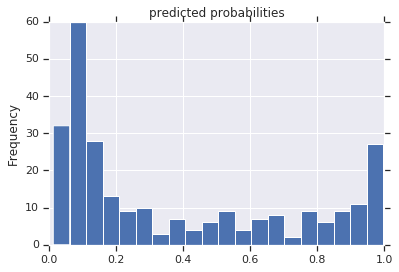
现在您可以使用训练的模型从评估集上对乘客进行预测了。Tensorflow 模型经过优化,可以同时在一个 batch 或一个集合的样本上进行预测。之前,eval_inout_fn 是使用整个评估集定义的。
pred_dicts = list(est.predict(eval_input_fn))
probs = pd.Series([pred['probabilities'][1] for pred in pred_dicts])

probs.plot(kind='hist', bins=20, title='predicted probabilities')
plt.show()
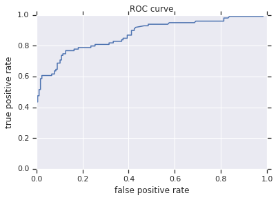
最后,您还可以查看结果的受试者工作特征曲线(ROC),这将使我们更好地了解真阳性率与假阴性率之间的权衡。
from sklearn.metrics import roc_curve

fpr, tpr, _ = roc_curve(y_eval, probs)
plt.plot(fpr, tpr)
plt.title('ROC curve')
plt.xlabel('false positive rate')
plt.ylabel('true positive rate')
plt.xlim(0,)
plt.ylim(0,)
plt.show()