
| |
|
 GitHub에서 소스 보기 GitHub에서 소스 보기 |
소개
이 노트북은 TensorFlow Core 하위 수준 API를 사용하여 고성능 과학적 컴퓨팅 플랫폼으로서의 TensorFlow의 기능을 보여줍니다. TensorFlow Core 및 기본 사용 사례에 대한 자세한 내용은 Core API 개요를 방문하여 확인하세요.
이 튜토리얼에서는 특잇값 분해(SVD) 기술과 낮은 순위의 근삿값 문제에 대한 적용을 살펴봅니다. SVD는 실수 혹은 복소수 행렬을 인수분해하는 데 사용하며 이미지 압축과 같은 데이터 과학에서 다양한 사용 사례가 있습니다. 이 튜토리얼의 이미지는 Google Brain의 Imagen 프로젝트에서 가져왔습니다.
설치하기
import matplotlib
from matplotlib.image import imread
from matplotlib import pyplot as plt
import requests
# Preset Matplotlib figure sizes.
matplotlib.rcParams['figure.figsize'] = [16, 9]
import tensorflow as tf
print(tf.__version__)
2022-12-14 21:32:31.375628: W tensorflow/compiler/xla/stream_executor/platform/default/dso_loader.cc:64] Could not load dynamic library 'libnvinfer.so.7'; dlerror: libnvinfer.so.7: cannot open shared object file: No such file or directory
2022-12-14 21:32:31.375727: W tensorflow/compiler/xla/stream_executor/platform/default/dso_loader.cc:64] Could not load dynamic library 'libnvinfer_plugin.so.7'; dlerror: libnvinfer_plugin.so.7: cannot open shared object file: No such file or directory
2022-12-14 21:32:31.375736: W tensorflow/compiler/tf2tensorrt/utils/py_utils.cc:38] TF-TRT Warning: Cannot dlopen some TensorRT libraries. If you would like to use Nvidia GPU with TensorRT, please make sure the missing libraries mentioned above are installed properly.
2.11.0
SVD 기본 사항
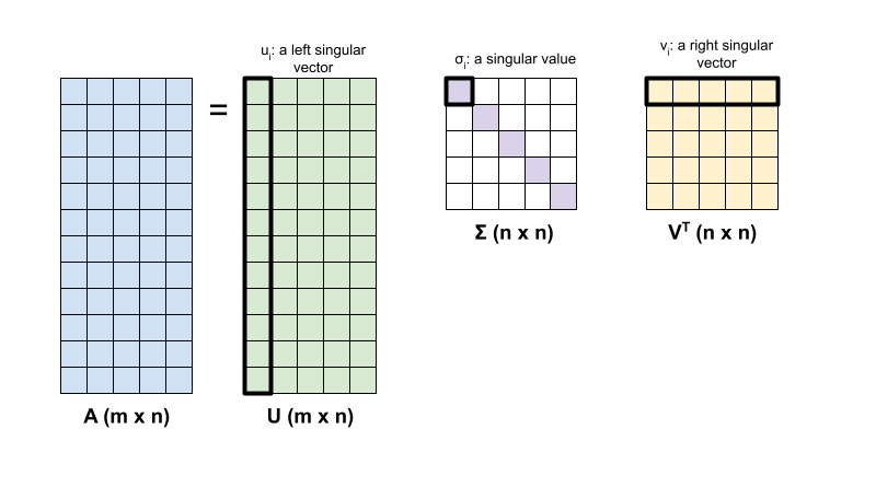
행렬 \({\mathrm{A} }\)의 특잇값 분해는 다음 인수분해에 의해 결정됩니다.
\[{\mathrm{A} } = {\mathrm{U} } \Sigma {\mathrm{V} }^T\]
여기서,
- \(\underset{m \times n}{\mathrm{A} }\): \(m \geq n\)인 입력 행렬
- \(\underset{m \times n}{\mathrm{U} }\): 직교 행렬, \({\mathrm{U} }^T{\mathrm{U} } = {\mathrm{I} }\), 각 열에서, \(u_i\), \({\mathrm{A} }\)의 왼쪽 특이 벡터를 나타냄
- \(\underset{n \times n}{\Sigma}\): \({\mathrm{A} }\)의 특이값을 나타내는 각 대각 입력 항목 \(\sigma_i\)가 있는 대각 행렬
- \(\underset{n \times n}{ {\mathrm{V} }^T}\): 직교 행렬, \({\mathrm{V} }^T{\mathrm{V} } = {\mathrm{I} }\), 각 행에 \(v_i\), \({\mathrm{A} }\)의 오른쪽 특이 벡터를 나타냄
\(m < n\)일 때 \({\mathrm{U} }\) 및 \(\Sigma\)은 모두 \((m \times m)\) 차원이며 \({\mathrm{V} }^T\)는 \((m \times n)\) 차원을 가짐.
TensorFlow의 선형 대수 패키지에는 하나 이상의 행렬의 특잇값 분해를 계산하는 데 사용할 수 있는 tf.linalg.svd 함수가 있습니다. 먼저 간단한 행렬을 정의하고 SVD 인수분해를 계산하는 것으로 시작합니다.
A = tf.random.uniform(shape=[40,30])
# Compute the SVD factorization
s, U, V = tf.linalg.svd(A)
# Define Sigma and V Transpose
S = tf.linalg.diag(s)
V_T = tf.transpose(V)
# Reconstruct the original matrix
A_svd = U@S@V_T
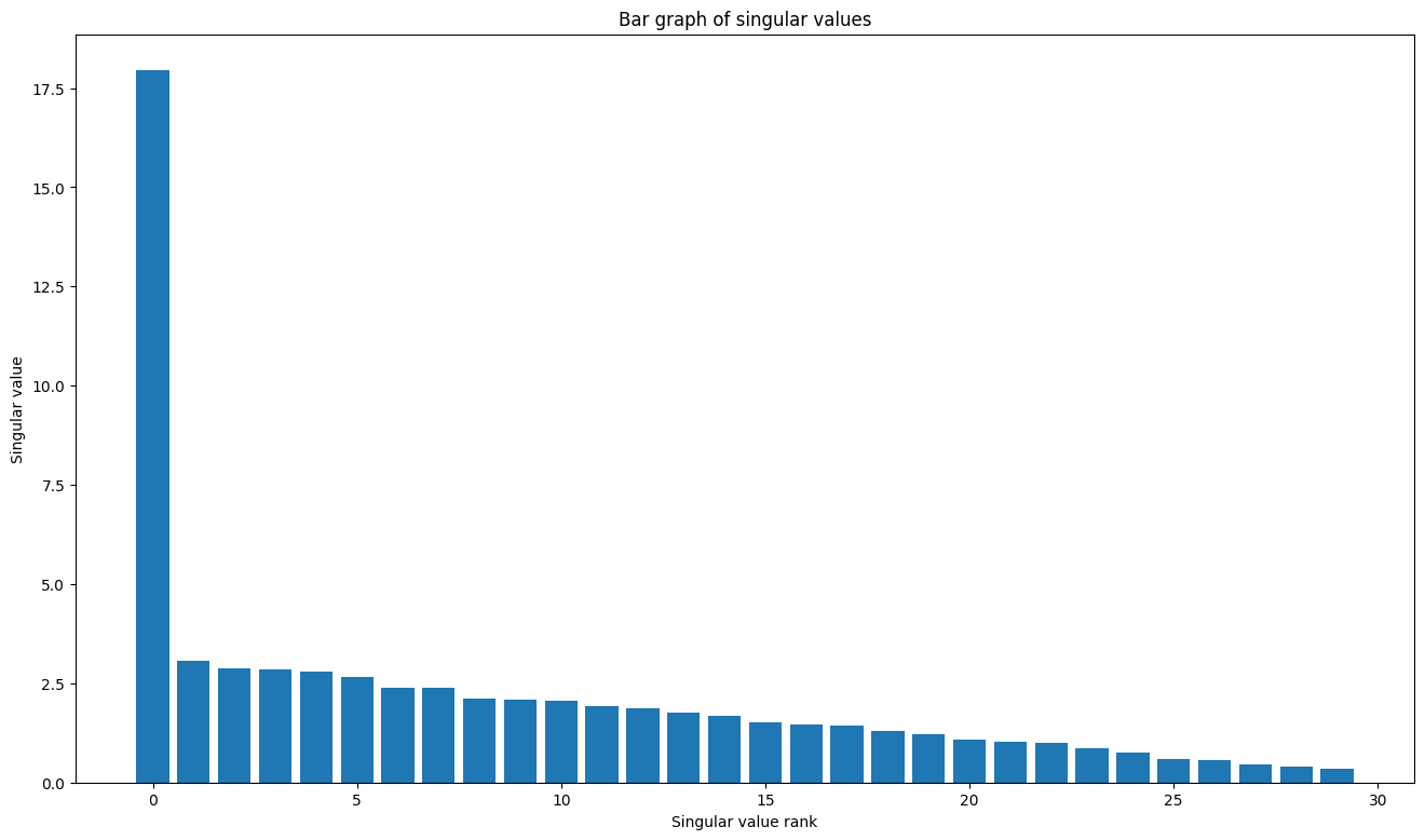
# Visualize
plt.bar(range(len(s)), s);
plt.xlabel("Singular value rank")
plt.ylabel("Singular value")
plt.title("Bar graph of singular values");
tf.linalg.svd의 출력에서 행렬 재구성을 직접 계산하는 경우 tf.einsum 함수를 사용할 수 있습니다.
A_svd = tf.einsum('s,us,vs -> uv',s,U,V)
print('\nReconstructed Matrix, A_svd', A_svd)
Reconstructed Matrix, A_svd tf.Tensor(
[[0.20475924 0.1842995  0.8591781  ... 0.7081913  0.62863785 0.5829904 ]
 [0.5544156  0.9010906  0.23621707 ... 0.55478156 0.35417116 0.8789251 ]
 [0.18557303 0.8689864  0.1450682  ... 0.02186572 0.06030737 0.40164167]
 ...
 [0.86776364 0.21518077 0.6085125  ... 0.33427155 0.68408597 0.45636302]
 [0.1923095  0.48697326 0.03344846 ... 0.1944161  0.67882144 0.59628713]
 [0.11751349 0.7671342  0.97516614 ... 0.4782539  0.21316503 0.12817305]], shape=(40, 30), dtype=float32)
SVD를 사용하는 낮은 순위 근삿값
행렬의 순위 \({\mathrm{A} }\)는 열에 걸쳐 있는 벡터 공간의 차원에 의해 결정됩니다. SVD는 더 낮은 순위의 행렬 근삿값을 계산하는 데 사용할 수 있으며, 이는 궁극적으로 행렬이 나타내는 정보를 저장하는 데 필요한 데이터의 차원수를 감소시킵니다.
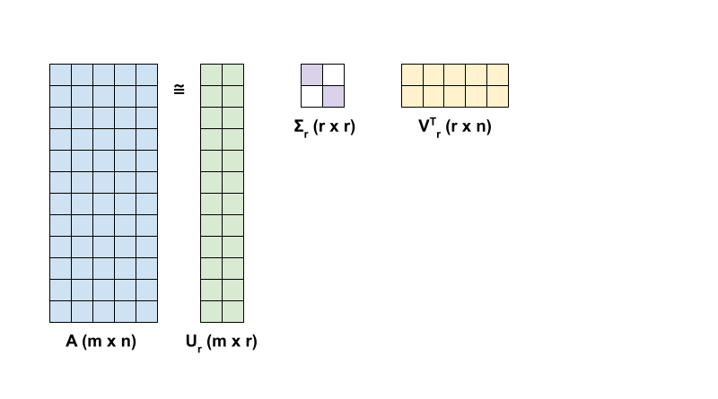
SVD의 관점에서 \({\mathrm{A} }\)의 rank-r 근삿값은 다음 공식으로 정의합니다.
\[{\mathrm{A_r} } = {\mathrm{U_r} } \Sigma_r {\mathrm{V_r} }^T\]
여기서,
- \(\underset{m \times r}{\mathrm{U_r} }\): \({\mathrm{U} }\)의 첫 번째 \(r\) 열로 구성된 행렬
- \(\underset{r \times r}{\Sigma_r}\): \(\Sigma\)의 첫 번째 \(r\) 특잇값으로 구성된 대각 행렬
- \(\underset{r \times n}{\mathrm{V_r} }^T\): \({\mathrm{V} }^T\)의 처음 \(r\) 행으로 구성된 행렬
먼저 주어진 행렬의 rank-r 근삿값을 계산하는 함수를 작성합니다. 이 낮은 순위 근삿값 계산 절차는 이미지 압축에 사용됩니다. 따라서 각 근삿값의 물리적 데이터 크기를 계산하는 것도 도움이 됩니다. 간단하게 하기 위해 rank-r 근사 행렬의 데이터 크기가 근삿값을 계산하는 데 필요한 총 요소의 수와 같다고 가정합니다. 그 다음에는 원래 행렬 \(\mathrm{A}\)와 이에 해당하는 rank-r 근삿값 \(\mathrm{A}_r\) 및 오류 행렬 \(|\mathrm{A} - \mathrm{A}_r|\)를 시각화하는 함수를 작성합니다.
def rank_r_approx(s, U, V, r, verbose=False):
  # Compute the matrices necessary for a rank-r approximation
  s_r, U_r, V_r = s[..., :r], U[..., :, :r], V[..., :, :r] # ... implies any number of extra batch axes
  # Compute the low-rank approximation and its size
  A_r = tf.einsum('...s,...us,...vs->...uv',s_r,U_r,V_r)
  A_r_size = tf.size(U_r) + tf.size(s_r) + tf.size(V_r)
  if verbose:
    print(f"Approximation Size: {A_r_size}")
  return A_r, A_r_size

def viz_approx(A, A_r):
  # Plot A, A_r, and A - A_r
  vmin, vmax = 0, tf.reduce_max(A)
  fig, ax = plt.subplots(1,3)
  mats = [A, A_r, abs(A - A_r)]
  titles = ['Original A', 'Approximated A_r', 'Error |A - A_r|']
  for i, (mat, title) in enumerate(zip(mats, titles)):
    ax[i].pcolormesh(mat, vmin=vmin, vmax=vmax)
    ax[i].set_title(title)
    ax[i].axis('off')
print(f"Original Size of A: {tf.size(A)}")
s, U, V = tf.linalg.svd(A)
Original Size of A: 1200
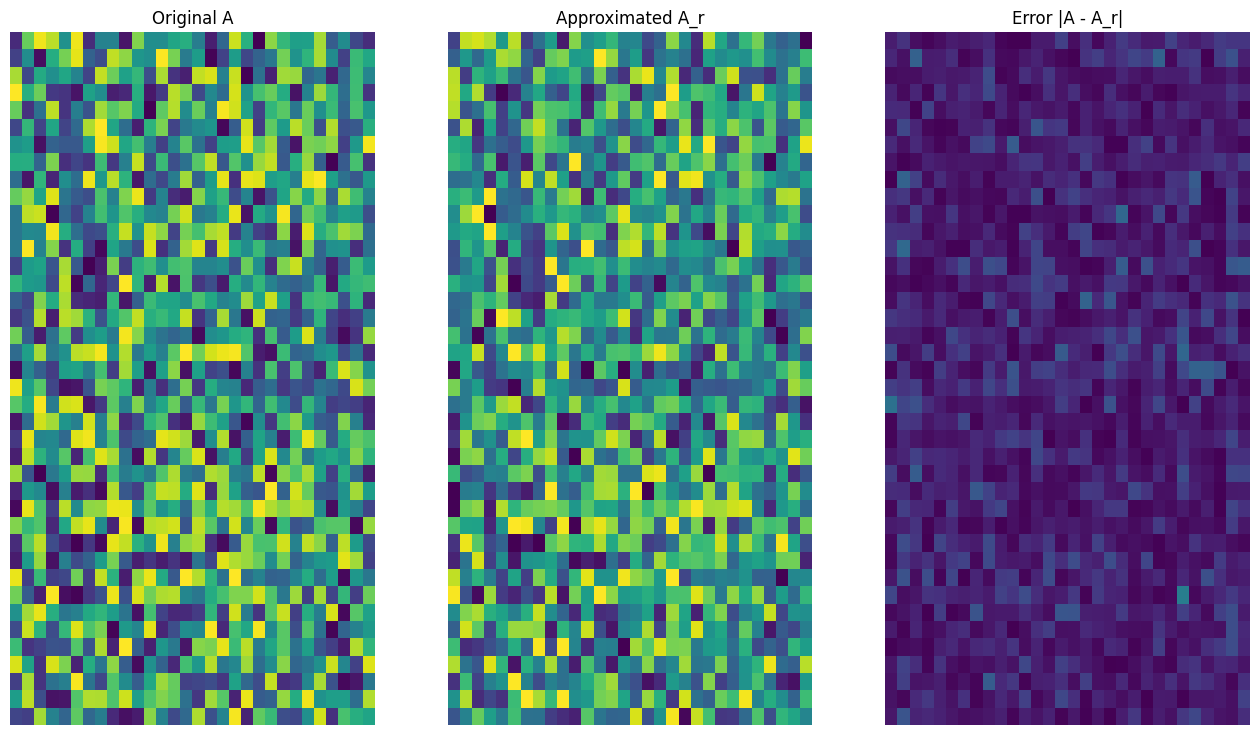
# Rank-15 approximation
A_15, A_15_size = rank_r_approx(s, U, V, 15, verbose = True)
viz_approx(A, A_15)
Approximation Size: 1065
# Rank-3 approximation
A_3, A_3_size = rank_r_approx(s, U, V, 3, verbose = True)
viz_approx(A, A_3)
Approximation Size: 213
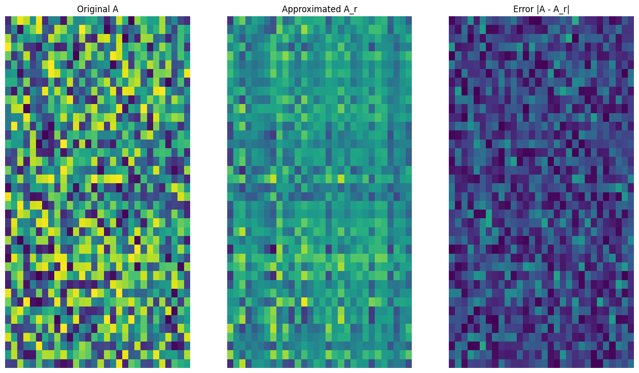
예상대로 낮은 순위를 사용하면 근삿값이 덜 정확해집니다. 그러나 이러한 낮은 순위 근삿값의 품질이 실제 시나리오에서는 충분히 좋은 경우가 있습니다. 또한 SVD를 사용하는 낮은 순위 근삿값의 주요 목표는 데이터의 차원수를 줄이는 것이며, 데이터 자체의 디스크 공간을 줄이는 것은 아닙니다. 다만 입력 행렬이 고차원이 될수록 많은 낮은 순위 근삿값도 데이터 크기 감소의 이점을 얻게 됩니다. 이러한 감소 이점이 프로세스를 이미지 압축 문제에 적용할 수 있는 이유입니다.
이미지 로드하기
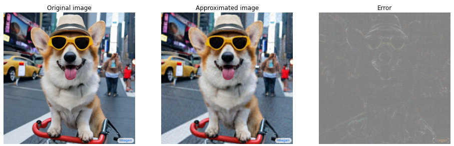
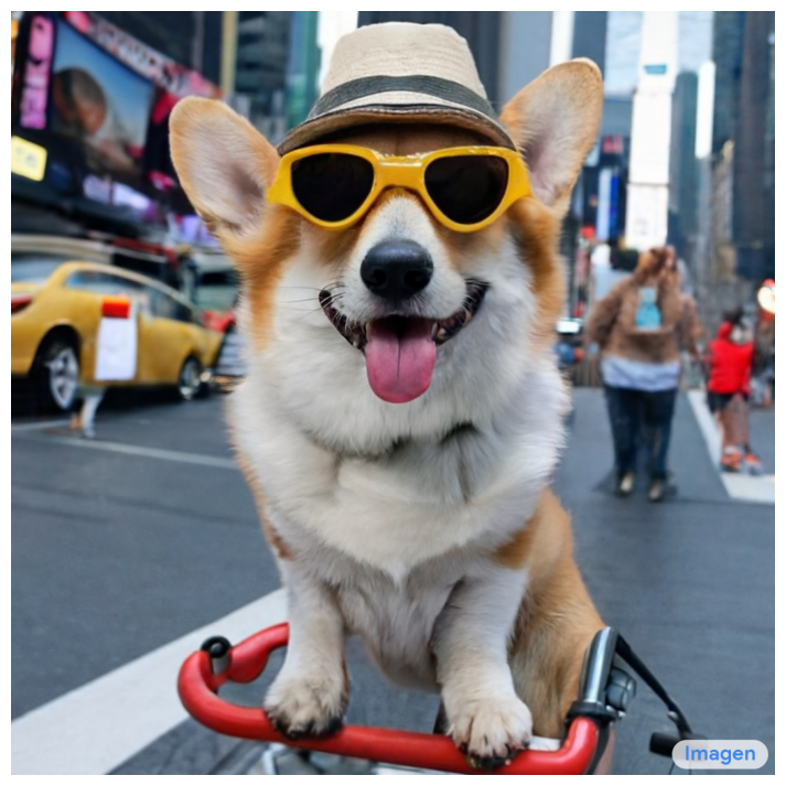
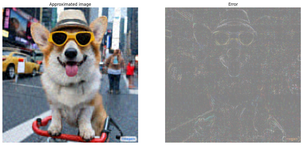
다음 이미지는 Imagen 홈페이지에서 사용할 수 있습니다. Imagen은 Google Research의 Brain 팀에서 개발한 텍스트-이미지 확산 모델입니다. "타임스퀘어에서 자전거를 타고 있는 Corgi 개 사진. 선글라스와 해변 모자를 쓰고 있습니다."라는 프롬프트를 기반으로 AI가 이 이미지를 생성했습니다. 얼마나 멋진 일인가요! 아래 URL을 .jpg 링크로 변경하여 선택한 사용자 정의 이미지를 로드할 수도 있습니다.
먼저 이미지를 읽고 시각화합니다. JPEG 파일을 읽어들인 후 Matplotlib가\((m \times n \times 3)\) 형상의 행렬 \({\mathrm{I} }\)을 출력합니다. 이 행렬은 각각 빨강, 초록, 파랑의 3개 색상 채널이 있는 2차원 이미지를 나타냅니다.
img_link = "https://imagen.research.google/main_gallery_images/a-photo-of-a-corgi-dog-riding-a-bike-in-times-square.jpg"
img_path = requests.get(img_link, stream=True).raw
I = imread(img_path, 0)
print("Input Image Shape:", I.shape)
Input Image Shape: (1024, 1024, 3)
def show_img(I):
  # Display the image in matplotlib
  img = plt.imshow(I)
  plt.axis('off')
  return
show_img(I)
이미지 압축 알고리즘
이제 SVD를 사용하여 샘플 이미지의 낮은 순위 근삿값을 계산합니다. 이미지의 형상이 \((1024 \times 1024 \times 3)\)이고 이론 SVD는 2차원 행렬에만 적용된다는 것을 기억해야 합니다. 이는 샘플 이미지가 3개의 색상 채널 각각에 해당하는 동일한 크기 행렬 3개로 배치되어야 함을 의미합니다. 이것은 행렬을 \((3 \times 1024 \times 1024)\) 형상으로 전치함으로써 수행할 수 있습니다. 근삿값 오차를 명확하게 시각화하기 위해 이미지의 RGB 값을 \([0,255]\)에서 \([0,1]\)로 다시 조정합니다. 근삿값을 시각화하기 전에 이 간격 안에 포함되도록 잘라내야 합니다. 이 작업에는 tf.clip_by_value 함수가 유용합니다.
def compress_image(I, r, verbose=False):
  # Compress an image with the SVD given a rank
  I_size = tf.size(I)
  print(f"Original size of image: {I_size}")
  # Compute SVD of image
  I = tf.convert_to_tensor(I)/255
  I_batched = tf.transpose(I, [2, 0, 1]) # einops.rearrange(I, 'h w c -> c h w')
  s, U, V = tf.linalg.svd(I_batched)
  # Compute low-rank approximation of image across each RGB channel
  I_r, I_r_size = rank_r_approx(s, U, V, r)
  I_r = tf.transpose(I_r, [1, 2, 0]) # einops.rearrange(I_r, 'c h w -> h w c')
  I_r_prop = (I_r_size / I_size)
  if verbose:
    # Display compressed image and attributes
    print(f"Number of singular values used in compression: {r}")
    print(f"Compressed image size: {I_r_size}")
    print(f"Proportion of original size: {I_r_prop:.3f}")
    ax_1 = plt.subplot(1,2,1)
    show_img(tf.clip_by_value(I_r,0.,1.))
    ax_1.set_title("Approximated image")
    ax_2 = plt.subplot(1,2,2)
    show_img(tf.clip_by_value(0.5+abs(I-I_r),0.,1.))
    ax_2.set_title("Error")
  return I_r, I_r_prop
이제 100, 50, 10 순위에 대한 rank-r 근삿값을 계산합니다.
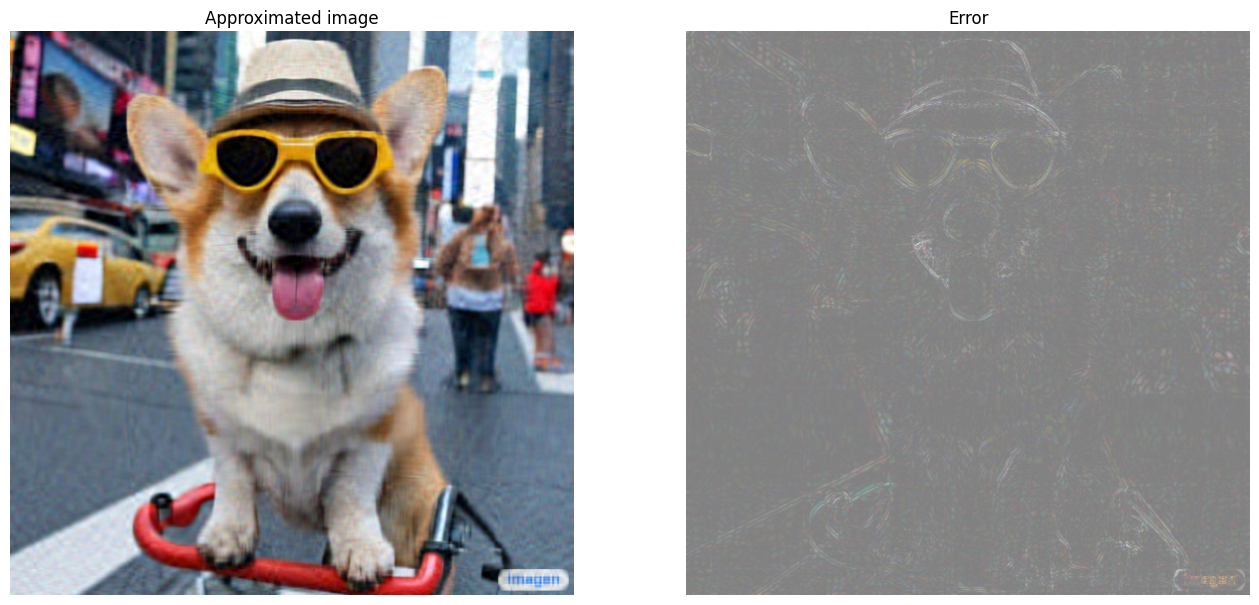
I_100, I_100_prop = compress_image(I, 100, verbose=True)
Original size of image: 3145728
Number of singular values used in compression: 100
Compressed image size: 614700
Proportion of original size: 0.195
I_50, I_50_prop = compress_image(I, 50, verbose=True)
Original size of image: 3145728
Number of singular values used in compression: 50
Compressed image size: 307350
Proportion of original size: 0.098
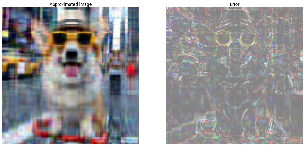
I_10, I_10_prop = compress_image(I, 10, verbose=True)
Original size of image: 3145728
Number of singular values used in compression: 10
Compressed image size: 61470
Proportion of original size: 0.020
근삿값 평가하기
효율성을 측정하고 행렬 근삿값을 더 잘 제어할 수 있는 다양하고 흥미로운 방법이 있습니다.
압축 인자 대 순위
위의 각 근삿값에 대해 순위에 따라 데이터 크기가 어떻게 변하는지 관찰해 보겠습니다.
plt.figure(figsize=(11,6))
plt.plot([100, 50, 10], [I_100_prop, I_50_prop, I_10_prop])
plt.xlabel("Rank")
plt.ylabel("Proportion of original image size")
plt.title("Compression factor vs rank");
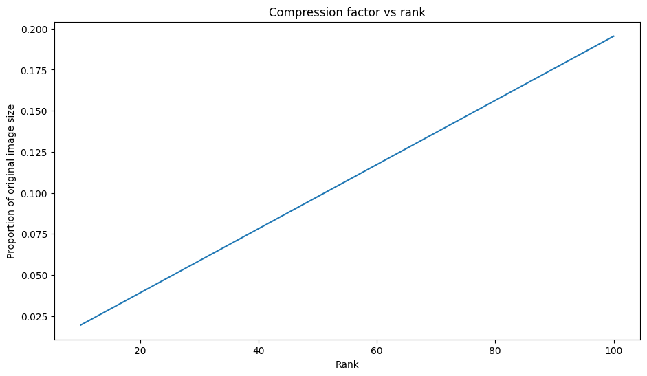
이 플롯을 기반으로 근삿값 이미지의 압축 인자와 순위 사이에는 선형 관계가 있습니다. 더 자세히 알아보기 위해 근삿값 행렬 \({\mathrm{A} }_r\)의 데이터 크기를 계산에 필요한 총 요소 수로 정의합니다. 다음 수식을 사용하여 압축 인자와 순위 사이의 관계를 찾을 수 있습니다.
\[x = (m \times r) + r + (r \times n) = r \times (m + n + 1)\]
\[c = \large \frac{x}{y} = \frac{r \times (m + n + 1)}{m \times n}\]
여기서,
- \(x\): \({\mathrm{A_r} }\)의 크기
- \(y\): \({\mathrm{A} }\)의 크기
- \(c = \frac{x}{y}\): 압축 인자
- \(r\): 근삿값의 순위
- \(m\) 와 \(n\): \({\mathrm{A} }\)의 행과 열 차원
이미지를 원하는 인자 \(c\)로 압축하는 데 필요한 순위 \(r\)를 찾기 위해 위의 수식을 다시 정렬하여 \(r\)를 풀이할 수 있습니다.
\[r = ⌊{\large\frac{c \times m \times n}{m + n + 1} }⌋\]
각 RGB 근삿값은 서로 영향을 미치지 않으므로 이 공식은 색상 채널 차원과 무관합니다. 이제 원하는 압축 인자가 주어질 경우 입력 이미지를 압축하는 함수를 작성합니다.
def compress_image_with_factor(I, compression_factor, verbose=False):
  # Returns a compressed image based on a desired compression factor
  m,n,o = I.shape
  r = int((compression_factor * m * n)/(m + n + 1))
  I_r, I_r_prop = compress_image(I, r, verbose=verbose)
  return I_r
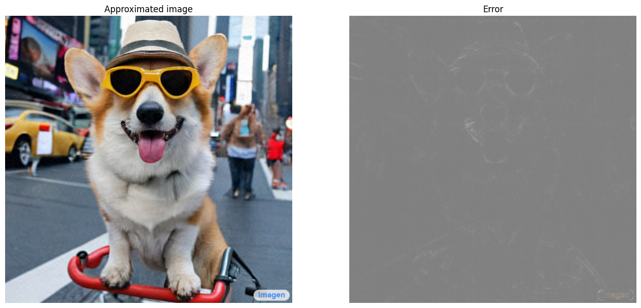
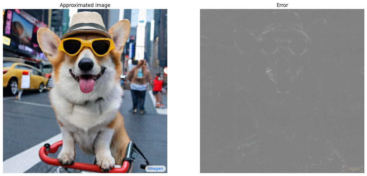
이미지를 원래 크기의 15%로 압축합니다.
compression_factor = 0.15
I_r_img = compress_image_with_factor(I, compression_factor, verbose=True)
Original size of image: 3145728
Number of singular values used in compression: 76
Compressed image size: 467172
Proportion of original size: 0.149
특잇값의 누적 합계
특잇값의 누적 합계는 rank-r 근삿값으로 캡처한 에너지 양에 대한 유용한 지표가 될 수 있습니다. 샘플 이미지 특잇값의 RGB 평균 누적 비율을 시각화합니다. 이러한 작업에 tf.cumsum 함수가 유용할 수 있습니다.
def viz_energy(I):
  # Visualize the energy captured based on rank
  # Computing SVD
  I = tf.convert_to_tensor(I)/255
  I_batched = tf.transpose(I, [2, 0, 1])
  s, U, V = tf.linalg.svd(I_batched)
  # Plotting average proportion across RGB channels
  props_rgb = tf.map_fn(lambda x: tf.cumsum(x)/tf.reduce_sum(x), s)
  props_rgb_mean = tf.reduce_mean(props_rgb, axis=0)
  plt.figure(figsize=(11,6))
  plt.plot(range(len(I)), props_rgb_mean, color='k')
  plt.xlabel("Rank / singular value number")
  plt.ylabel("Cumulative proportion of singular values")
  plt.title("RGB-averaged proportion of energy captured by the first 'r' singular values")
viz_energy(I)
WARNING:tensorflow:From /tmpfs/src/tf_docs_env/lib/python3.9/site-packages/tensorflow/python/autograph/pyct/static_analysis/liveness.py:83: Analyzer.lamba_check (from tensorflow.python.autograph.pyct.static_analysis.liveness) is deprecated and will be removed after 2023-09-23.
Instructions for updating:
Lambda fuctions will be no more assumed to be used in the statement where they are used, or at least in the same block. https://github.com/tensorflow/tensorflow/issues/56089
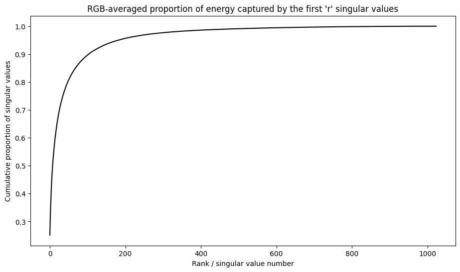
이 이미지의 에너지 중 90% 이상이 처음 100개의 특잇값 내에서 캡처된 것 같습니다. 이제 원하는 에너지 머무름 인자(retention factor)가 주어질 경우 입력 이미지를 압축하는 함수를 작성합니다.
def compress_image_with_energy(I, energy_factor, verbose=False):
  # Returns a compressed image based on a desired energy factor
  # Computing SVD
  I_rescaled = tf.convert_to_tensor(I)/255
  I_batched = tf.transpose(I_rescaled, [2, 0, 1])
  s, U, V = tf.linalg.svd(I_batched)
  # Extracting singular values
  props_rgb = tf.map_fn(lambda x: tf.cumsum(x)/tf.reduce_sum(x), s)
  props_rgb_mean = tf.reduce_mean(props_rgb, axis=0)
  # Find closest r that corresponds to the energy factor
  r = tf.argmin(tf.abs(props_rgb_mean - energy_factor)) + 1
  actual_ef = props_rgb_mean[r]
  I_r, I_r_prop = compress_image(I, r, verbose=verbose)
  print(f"Proportion of energy captured by the first {r} singular values: {actual_ef:.3f}")
  return I_r
75%의 이미지를 유지하기 위해 이미지를 압축합니다.
energy_factor = 0.75
I_r_img = compress_image_with_energy(I, energy_factor, verbose=True)
Original size of image: 3145728
Number of singular values used in compression: 35
Compressed image size: 215145
Proportion of original size: 0.068
Proportion of energy captured by the first 35 singular values: 0.753
오차와 특잇값
근삿값 오차와 특잇값 사이에도 흥미로운 상관 관계가 있습니다. 제곱한 프로베니우스 노름(Frobenius norm) 근삿값은 제외된 특잇값의 제곱의 합과 같다는 것이 밝혀졌습니다.
\[{||A - A_r||}^2 = \sum_{i=r+1}^{R}σ_i^2\]
이 튜토리얼의 시작 부분에 있는 예제 행렬의 10 순위 근삿값으로 이러한 관계를 테스트해보겠습니다.
s, U, V = tf.linalg.svd(A)
A_10, A_10_size = rank_r_approx(s, U, V, 10)
squared_norm = tf.norm(A - A_10)**2
s_squared_sum = tf.reduce_sum(s[10:]**2)
print(f"Squared Frobenius norm: {squared_norm:.3f}")
print(f"Sum of squared singular values left out: {s_squared_sum:.3f}")
Squared Frobenius norm: 32.689
Sum of squared singular values left out: 32.689
결론
이 노트북에서는 TensorFlow를 사용하는 특잇값 분해를 구현하고 이를 적용하여 이미지 압축 알고리즘을 작성하는 프로세스를 소개했습니다. 다음은 도움이 될 수 있는 몇 가지 추가 팁입니다.
- TensorFlow Core API를 다양한 고성능 과학적 컴퓨팅 사용 사례에 활용할 수 있습니다.
- TensorFlow의 선형 대수 기능에 대해 자세히 알아보려면 linalg 모듈 문서를 방문하여 확인하세요.
- SVD를 추천 시스템 빌드에도 적용할 수 있습니다.
TensorFlow Core API를 사용하는 더 많은 예제는 가이드를 확인하세요. 데이터 로드 및 준비에 대해 자세히 알아보려면 이미지 데이터 로드 또는 CSV 데이터 로드 튜토리얼을 참고하세요.