| | |  Xem nguồn trên GitHub Xem nguồn trên GitHub | |
Đây là cổng Xác suất TensorFlow của bài báo cùng tên ngày 16 tháng 3 năm 2020 của Li et al. Chúng tôi tái tạo trung thực các phương pháp và kết quả của tác giả gốc trên nền tảng Xác suất TensorFlow, thể hiện một số khả năng của TFP trong việc thiết lập mô hình dịch tễ học hiện đại. Việc chuyển sang TensorFlow cung cấp cho chúng tôi tốc độ tăng gấp ~ 10 lần so với mã Matlab ban đầu và, vì TensorFlow Probability hỗ trợ rộng rãi tính toán hàng loạt được vectơ hóa, nên cũng có thể mở rộng thành hàng trăm bản sao độc lập một cách thuận lợi.
Bản gốc
Ruiyun Li, Sen Pei, Bin Chen, Yimeng Song, Tao Zhang, Wan Yang và Jeffrey Shaman. Sự lây nhiễm đáng kể không có giấy tờ tạo điều kiện cho sự phổ biến nhanh chóng của coronavirus mới (SARS-CoV2). (2020), doi: https://doi.org/10.1126/science.abb3221 .
Tóm tắt:. "Ước tính tỷ lệ và contagiousness các bệnh nhiễm trùng tiểu thuyết coronavirus (SARS-CoV2) không có giấy tờ là rất quan trọng để hiểu được sự phổ biến tổng thể và tiềm năng đại dịch của bệnh này ở đây chúng tôi sử dụng quan sát nhiễm được báo cáo trong Trung Quốc, kết hợp với dữ liệu di động, một mô hình siêu nhân động được nối mạng và suy luận Bayes, để suy ra các đặc điểm dịch tễ học quan trọng liên quan đến SARS-CoV2, bao gồm cả phần nhỏ các ca nhiễm trùng không có giấy tờ và khả năng lây lan của chúng. Chúng tôi ước tính 86% tổng số ca nhiễm trùng không có giấy tờ (KTC 95%: [82% –90%] ) trước ngày 23 tháng 1 năm 2020 hạn chế đi lại. Tính theo người, tỷ lệ lây truyền các ca nhiễm trùng không có giấy tờ là 55% các ca nhiễm trùng được ghi nhận ([46% –62%]), tuy nhiên, do số lượng nhiều hơn, các ca nhiễm trùng không có giấy tờ là nguồn lây nhiễm cho 79 % các trường hợp được ghi nhận. Những phát hiện này giải thích sự lây lan nhanh chóng về mặt địa lý của SARS-CoV2 và cho thấy việc ngăn chặn loại vi rút này sẽ đặc biệt khó khăn. "
Github liên kết đến mã và dữ liệu.
Tổng quat
Mô hình này là một mô hình bệnh compartmental , với khoang cho "nhạy cảm", "tiếp xúc" (nhiễm nhưng chưa truyền nhiễm), "không bao giờ như các tài liệu truyền nhiễm", và "cuối cùng các tài liệu truyền nhiễm". Có hai đặc điểm đáng chú ý: các ngăn riêng biệt cho mỗi thành phố trong số 375 thành phố của Trung Quốc, với giả định về cách mọi người đi từ thành phố này sang thành phố khác; và sự chậm trễ trong việc báo cáo nhiễm trùng, do đó một trường hợp đó trở thành "cuối cùng các tài liệu truyền nhiễm" vào ngày \(t\) không hiển thị trong trường hợp số lượng quan sát cho đến khi một ngày sau đó ngẫu nhiên.
Mô hình giả định rằng các trường hợp không bao giờ được lập tài liệu sẽ không có tài liệu do nhẹ hơn và do đó lây nhiễm cho những người khác với tỷ lệ thấp hơn. Thông số chính được quan tâm trong tài liệu gốc là tỷ lệ các trường hợp không có giấy tờ, để ước tính cả mức độ lây nhiễm hiện có và tác động của việc lây truyền không có giấy tờ đối với sự lây lan của bệnh.
Chuyên mục này được cấu trúc như một hướng dẫn mã theo kiểu từ dưới lên. Để, chúng tôi sẽ
- Nhập và kiểm tra nhanh dữ liệu,
- Xác định không gian trạng thái và động lực của mô hình,
- Xây dựng một bộ chức năng để thực hiện suy luận trong mô hình theo Li và cộng sự, và
- Gọi họ và xem xét kết quả. Spoiler: Chúng xuất hiện giống như tờ giấy.
Cài đặt và nhập Python
pip3 install -q tf-nightly tfp-nightly
import collections
import io
import requests
import time
import zipfile

import matplotlib.pyplot as plt
import numpy as np
import pandas as pd

import tensorflow.compat.v2 as tf
import tensorflow_probability as tfp
from tensorflow_probability.python.internal import samplers

tfd = tfp.distributions
tfes = tfp.experimental.sequential
Nhập dữ liệu
Hãy nhập dữ liệu từ github và kiểm tra một số dữ liệu.
r = requests.get('https://raw.githubusercontent.com/SenPei-CU/COVID-19/master/Data.zip')
z = zipfile.ZipFile(io.BytesIO(r.content))
z.extractall('/tmp/')
raw_incidence = pd.read_csv('/tmp/data/Incidence.csv')
raw_mobility = pd.read_csv('/tmp/data/Mobility.csv')
raw_population = pd.read_csv('/tmp/data/pop.csv')
Dưới đây, chúng ta có thể thấy số lượng tỷ lệ mắc bệnh thô mỗi ngày. Chúng tôi quan tâm nhất đến 14 ngày đầu tiên (từ ngày 10 tháng 1 đến ngày 23 tháng 1), vì các hạn chế đi lại được đưa ra vào ngày 23. Bài báo giải quyết vấn đề này bằng cách lập mô hình ngày 10-23 tháng 1 và ngày 23 tháng 1 trở lên riêng biệt, với các thông số khác nhau; chúng tôi sẽ chỉ hạn chế tái sản xuất của chúng tôi trong khoảng thời gian trước đó.
raw_incidence.drop('Date', axis=1)  # The 'Date' column is all 1/18/21
# Luckily the days are in order, starting on January 10th, 2020.
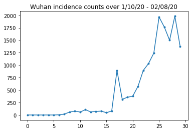
Hãy tỉnh táo kiểm tra số lượng tỷ lệ mắc bệnh ở Vũ Hán.
plt.plot(raw_incidence.Wuhan, '.-')
plt.title('Wuhan incidence counts over 1/10/20 - 02/08/20')
plt.show()
Càng xa càng tốt. Bây giờ dân số ban đầu được tính.
raw_population
Hãy cũng kiểm tra và ghi lại mục nhập nào là Vũ Hán.
raw_population['City'][169]
'Wuhan'
WUHAN_IDX = 169
Và ở đây chúng ta thấy ma trận di chuyển giữa các thành phố khác nhau. Đây là đại diện cho số lượng người di chuyển giữa các thành phố khác nhau trong 14 ngày đầu tiên. Nó được lấy từ các bản ghi GPS do Tencent cung cấp cho mùa Tết Nguyên đán 2018. Li et al mô hình di động trong mùa 2020 như một số không rõ (tùy thuộc vào suy luận) yếu tố liên tục \(\theta\) lần này.
raw_mobility
Cuối cùng, hãy xử lý trước tất cả những điều này thành các mảng numpy mà chúng ta có thể sử dụng.
# The given populations are only "initial" because of intercity mobility during
# the holiday season.
initial_population = raw_population['Population'].to_numpy().astype(np.float32)
Chuyển đổi dữ liệu di động thành Tensor hình [L, L, T], trong đó L là số vị trí và T là số bước thời gian.
daily_mobility_matrices = []
for i in range(1, 15):
  day_mobility = raw_mobility[raw_mobility['Day'] == i]

  # Make a matrix of daily mobilities.
  z = pd.crosstab(
      day_mobility.Origin,
      day_mobility.Destination,
      values=day_mobility['Mobility Index'], aggfunc='sum', dropna=False)

  # Include every city, even if there are no rows for some in the raw data on
  # some day.  This uses the sort order of `raw_population`.
  z = z.reindex(index=raw_population['City'], columns=raw_population['City'],
                fill_value=0)
  # Finally, fill any missing entries with 0. This means no mobility.
  z = z.fillna(0)
  daily_mobility_matrices.append(z.to_numpy())

mobility_matrix_over_time = np.stack(daily_mobility_matrices, axis=-1).astype(
    np.float32)
Cuối cùng lấy các nhiễm trùng quan sát được và lập bảng [L, T].
# Remove the date parameter and take the first 14 days.
observed_daily_infectious_count = raw_incidence.to_numpy()[:14, 1:]
observed_daily_infectious_count = np.transpose(
    observed_daily_infectious_count).astype(np.float32)
Và kiểm tra kỹ xem chúng ta đã có được các hình dạng theo cách chúng ta muốn chưa. Xin nhắc lại, chúng tôi đang làm việc với 375 thành phố và 14 ngày.
print('Mobility Matrix over time should have shape (375, 375, 14): {}'.format(
    mobility_matrix_over_time.shape))
print('Observed Infectious should have shape (375, 14): {}'.format(
    observed_daily_infectious_count.shape))
print('Initial population should have shape (375): {}'.format(
    initial_population.shape))
Mobility Matrix over time should have shape (375, 375, 14): (375, 375, 14)
Observed Infectious should have shape (375, 14): (375, 14)
Initial population should have shape (375): (375,)
Xác định trạng thái và thông số
Hãy bắt đầu xác định mô hình của chúng tôi. Mô hình chúng ta đang tái tạo là một biến thể của một mô hình Sê -i-rơ . Trong trường hợp này, chúng tôi có các trạng thái thay đổi theo thời gian sau:
- \(S\): Số người nhạy cảm với các bệnh ở mỗi thành phố.
- \(E\): Số người trong mỗi thành phố tiếp xúc với bệnh truyền nhiễm nhưng không được nêu ra. Về mặt sinh học, điều này tương ứng với việc lây nhiễm căn bệnh, trong đó tất cả những người bị phơi nhiễm cuối cùng đều bị lây nhiễm.
- \(I^u\): Số người trong mỗi thành phố người nhiễm nhưng không có cơ sở. Trong mô hình, điều này thực sự có nghĩa là "sẽ không bao giờ được ghi lại".
- \(I^r\): Số người trong mỗi thành phố những người nhiễm và ghi nhận như vậy. Li et al mô hình báo cáo chậm trễ, vì vậy \(I^r\) thực sự tương ứng với một cái gì đó như "trường hợp là đủ nghiêm trọng để được ghi nhận tại một số điểm trong tương lai".
Như chúng ta sẽ thấy bên dưới, chúng ta sẽ suy ra những trạng thái này bằng cách chạy Bộ lọc Kalman được điều chỉnh bởi Ensemble (EAKF) kịp thời. Vectơ trạng thái của EAKF là một vectơ được lập chỉ mục thành phố cho mỗi đại lượng này.
Mô hình có các tham số toàn cục, bất biến theo thời gian có thể suy ra được sau đây:
- \(\beta\): Tốc độ truyền do các cá nhân nhiễm trùng tài liệu.
- \(\mu\): Tốc độ truyền tương đối do cá nhân không có giấy tờ nhiễm trùng. Này sẽ hoạt động thông qua các sản phẩm \(\mu \beta\).
- \(\theta\): Các yếu tố liên tỉnh di động. Đây là hệ số lớn hơn 1 điều chỉnh đối với việc báo cáo thiếu dữ liệu về di chuyển (và đối với sự gia tăng dân số từ năm 2018 đến năm 2020).
- \(Z\): Thời gian ủ bệnh trung bình (ví dụ, thời gian trong "tiếp xúc" nhà nước).
- \(\alpha\): Đây là phần của nhiễm trùng đủ để thể nặng (cuối cùng) ghi nhận.
- \(D\): Thời lượng trung bình các bệnh nhiễm trùng (ví dụ, thời gian ở một trong hai trạng thái "nhiễm").
Chúng tôi sẽ suy ra các ước tính điểm cho các tham số này với một vòng lặp lặp lại bộ lọc xung quanh EAKF cho các trạng thái.
Mô hình cũng phụ thuộc vào các hằng số không được suy ra:
- \(M\): Ma trận liên tỉnh di động. Điều này thay đổi theo thời gian và được cho là đã đưa ra. Nhớ lại rằng nó thu nhỏ lại bởi những suy ra tham số \(\theta\) để cung cấp cho các phong trào dân số thực tế giữa các thành phố.
- \(N\): Tổng số người trong mỗi thành phố. Quần ban đầu được thực hiện như được đưa ra, và thời gian biến động dân số được tính toán từ các số di động \(\theta M\).
Đầu tiên, chúng tôi cung cấp cho mình một số cấu trúc dữ liệu để giữ các trạng thái và tham số của chúng tôi.
SEIRComponents = collections.namedtuple(
  typename='SEIRComponents',
  field_names=[
    'susceptible',              # S
    'exposed',                  # E
    'documented_infectious',    # I^r
    'undocumented_infectious',  # I^u
    # This is the count of new cases in the "documented infectious" compartment.
    # We need this because we will introduce a reporting delay, between a person
    # entering I^r and showing up in the observable case count data.
    # This can't be computed from the cumulative `documented_infectious` count,
    # because some portion of that population will move to the 'recovered'
    # state, which we aren't tracking explicitly.
    'daily_new_documented_infectious'])

ModelParams = collections.namedtuple(
    typename='ModelParams',
    field_names=[
      'documented_infectious_tx_rate',             # Beta
      'undocumented_infectious_tx_relative_rate',  # Mu
      'intercity_underreporting_factor',           # Theta
      'average_latency_period',                    # Z
      'fraction_of_documented_infections',         # Alpha
      'average_infection_duration'                 # D
    ]
)
Chúng tôi cũng mã hóa các giới hạn của Li et al cho các giá trị của các tham số.
PARAMETER_LOWER_BOUNDS = ModelParams(
    documented_infectious_tx_rate=0.8,
    undocumented_infectious_tx_relative_rate=0.2,
    intercity_underreporting_factor=1.,
    average_latency_period=2.,
    fraction_of_documented_infections=0.02,
    average_infection_duration=2.
)

PARAMETER_UPPER_BOUNDS = ModelParams(
    documented_infectious_tx_rate=1.5,
    undocumented_infectious_tx_relative_rate=1.,
    intercity_underreporting_factor=1.75,
    average_latency_period=5.,
    fraction_of_documented_infections=1.,
    average_infection_duration=5.
)
SEIR Dynamics
Ở đây chúng tôi xác định mối quan hệ giữa các tham số và trạng thái.
Các phương trình động lực học theo thời gian từ Li và cộng sự (tài liệu bổ sung, phương trình 1-5) như sau:
\(\frac{dS_i}{dt} = -\beta \frac{S_i I_i^r}{N_i} - \mu \beta \frac{S_i I_i^u}{N_i} + \theta \sum_k \frac{M_{ij} S_j}{N_j - I_j^r} - + \theta \sum_k \frac{M_{ji} S_j}{N_i - I_i^r}\)
\(\frac{dE_i}{dt} = \beta \frac{S_i I_i^r}{N_i} + \mu \beta \frac{S_i I_i^u}{N_i} -\frac{E_i}{Z} + \theta \sum_k \frac{M_{ij} E_j}{N_j - I_j^r} - + \theta \sum_k \frac{M_{ji} E_j}{N_i - I_i^r}\)
\(\frac{dI^r_i}{dt} = \alpha \frac{E_i}{Z} - \frac{I_i^r}{D}\)
\(\frac{dI^u_i}{dt} = (1 - \alpha) \frac{E_i}{Z} - \frac{I_i^u}{D} + \theta \sum_k \frac{M_{ij} I_j^u}{N_j - I_j^r} - + \theta \sum_k \frac{M_{ji} I^u_j}{N_i - I_i^r}\)
\(N_i = N_i + \theta \sum_j M_{ij} - \theta \sum_j M_{ji}\)
Xin nhắc lại, các \(i\) và \(j\) thành phố subscript chỉ mục. Các phương trình này mô hình hóa sự tiến triển theo thời gian của bệnh thông qua
- Tiếp xúc với các cá nhân lây nhiễm dẫn đến lây nhiễm nhiều hơn;
- Tiến triển của bệnh từ "tiếp xúc" sang một trong các trạng thái "lây nhiễm";
- Sự tiến triển của bệnh từ trạng thái "lây nhiễm" sang trạng thái phục hồi, mà chúng tôi lập mô hình bằng cách loại bỏ khỏi quần thể được lập mô hình;
- Di chuyển giữa các thành phố, bao gồm cả những người bị lây nhiễm tiếp xúc hoặc không có giấy tờ tùy thân; và
- Sự thay đổi theo thời gian của dân số thành phố hàng ngày thông qua sự di chuyển giữa các thành phố.
Theo Li và cộng sự, chúng tôi giả định rằng những người có ca bệnh đủ nghiêm trọng để cuối cùng được báo cáo không đi du lịch giữa các thành phố.
Cũng theo Li và cộng sự, chúng tôi coi các động lực này là đối tượng của nhiễu Poisson theo thuật ngữ, tức là, mỗi số hạng thực sự là tốc độ của một Poisson, một mẫu mà từ đó đưa ra sự thay đổi thực sự. Nhiễu Poisson là khôn ngoan vì việc trừ (trái ngược với cộng) các mẫu Poisson không mang lại kết quả có phân phối Poisson.
Chúng tôi sẽ phát triển những động lực học này về phía trước với bộ tích phân Runge-Kutta bậc 4 cổ điển, nhưng trước tiên hãy xác định hàm tính toán chúng (bao gồm cả lấy mẫu nhiễu Poisson).
def sample_state_deltas(
    state, population, mobility_matrix, params, seed, is_deterministic=False):
  """Computes one-step change in state, including Poisson sampling.

  Note that this is coded to support vectorized evaluation on arbitrary-shape
  batches of states.  This is useful, for example, for running multiple
  independent replicas of this model to compute credible intervals for the
  parameters.  We refer to the arbitrary batch shape with the conventional
  `B` in the parameter documentation below.  This function also, of course,
  supports broadcasting over the batch shape.

  Args:
    state: A `SEIRComponents` tuple with fields Tensors of shape
      B + [num_locations] giving the current disease state.
    population: A Tensor of shape B + [num_locations] giving the current city
      populations.
    mobility_matrix: A Tensor of shape B + [num_locations, num_locations] giving
      the current baseline inter-city mobility.
    params: A `ModelParams` tuple with fields Tensors of shape B giving the
      global parameters for the current EAKF run.
    seed: Initial entropy for pseudo-random number generation.  The Poisson
      sampling is repeatable by supplying the same seed.
    is_deterministic: A `bool` flag to turn off Poisson sampling if desired.

  Returns:
    delta: A `SEIRComponents` tuple with fields Tensors of shape
      B + [num_locations] giving the one-day changes in the state, according
      to equations 1-4 above (including Poisson noise per Li et al).
  """
  undocumented_infectious_fraction = state.undocumented_infectious / population
  documented_infectious_fraction = state.documented_infectious / population

  # Anyone not documented as infectious is considered mobile
  mobile_population = (population - state.documented_infectious)
  def compute_outflow(compartment_population):
    raw_mobility = tf.linalg.matvec(
        mobility_matrix, compartment_population / mobile_population)
    return params.intercity_underreporting_factor * raw_mobility
  def compute_inflow(compartment_population):
    raw_mobility = tf.linalg.matmul(
        mobility_matrix,
        (compartment_population / mobile_population)[..., tf.newaxis],
        transpose_a=True)
    return params.intercity_underreporting_factor * tf.squeeze(
        raw_mobility, axis=-1)

  # Helper for sampling the Poisson-variate terms.
  seeds = samplers.split_seed(seed, n=11)
  if is_deterministic:
    def sample_poisson(rate):
      return rate
  else:
    def sample_poisson(rate):
      return tfd.Poisson(rate=rate).sample(seed=seeds.pop())

  # Below are the various terms called U1-U12 in the paper. We combined the
  # first two, which should be fine; both are poisson so their sum is too, and
  # there's no risk (as there could be in other terms) of going negative.
  susceptible_becoming_exposed = sample_poisson(
      state.susceptible *
      (params.documented_infectious_tx_rate *
       documented_infectious_fraction +
       (params.undocumented_infectious_tx_relative_rate *
        params.documented_infectious_tx_rate) *
       undocumented_infectious_fraction))  # U1 + U2

  susceptible_population_inflow = sample_poisson(
      compute_inflow(state.susceptible))  # U3
  susceptible_population_outflow = sample_poisson(
      compute_outflow(state.susceptible))  # U4

  exposed_becoming_documented_infectious = sample_poisson(
      params.fraction_of_documented_infections *
      state.exposed / params.average_latency_period)  # U5
  exposed_becoming_undocumented_infectious = sample_poisson(
      (1 - params.fraction_of_documented_infections) *
      state.exposed / params.average_latency_period)  # U6

  exposed_population_inflow = sample_poisson(
      compute_inflow(state.exposed))  # U7
  exposed_population_outflow = sample_poisson(
      compute_outflow(state.exposed))  # U8

  documented_infectious_becoming_recovered = sample_poisson(
      state.documented_infectious /
      params.average_infection_duration)  # U9
  undocumented_infectious_becoming_recovered = sample_poisson(
      state.undocumented_infectious /
      params.average_infection_duration)  # U10

  undocumented_infectious_population_inflow = sample_poisson(
      compute_inflow(state.undocumented_infectious))  # U11
  undocumented_infectious_population_outflow = sample_poisson(
      compute_outflow(state.undocumented_infectious))  # U12

  # The final state_deltas
  return SEIRComponents(
      # Equation [1]
      susceptible=(-susceptible_becoming_exposed +
                   susceptible_population_inflow +
                   -susceptible_population_outflow),
      # Equation [2]
      exposed=(susceptible_becoming_exposed +
               -exposed_becoming_documented_infectious +
               -exposed_becoming_undocumented_infectious +
               exposed_population_inflow +
               -exposed_population_outflow),
      # Equation [3]
      documented_infectious=(
          exposed_becoming_documented_infectious +
          -documented_infectious_becoming_recovered),
      # Equation [4]
      undocumented_infectious=(
          exposed_becoming_undocumented_infectious +
          -undocumented_infectious_becoming_recovered +
          undocumented_infectious_population_inflow +
          -undocumented_infectious_population_outflow),
      # New to-be-documented infectious cases, subject to the delayed
      # observation model.
      daily_new_documented_infectious=exposed_becoming_documented_infectious)
Đây là bộ tích hợp. Điều này hoàn toàn tiêu chuẩn, trừ đi qua các hạt PRNG thông qua các sample_state_deltas chức năng để có được độc lập tiếng ồn Poisson tại từng bước một phần rằng phương pháp Runge-Kutta kêu gọi.
@tf.function(autograph=False)
def rk4_one_step(state, population, mobility_matrix, params, seed):
  """Implement one step of RK4, wrapped around a call to sample_state_deltas."""
  # One seed for each RK sub-step
  seeds = samplers.split_seed(seed, n=4)

  deltas = tf.nest.map_structure(tf.zeros_like, state)
  combined_deltas = tf.nest.map_structure(tf.zeros_like, state)

  for a, b in zip([1., 2, 2, 1.], [6., 3., 3., 6.]):
    next_input = tf.nest.map_structure(
        lambda x, delta, a=a: x + delta / a, state, deltas)
    deltas = sample_state_deltas(
        next_input,
        population,
        mobility_matrix,
        params,
        seed=seeds.pop(), is_deterministic=False)
    combined_deltas = tf.nest.map_structure(
        lambda x, delta, b=b: x + delta / b, combined_deltas, deltas)

  return tf.nest.map_structure(
      lambda s, delta: s + tf.round(delta),
      state, combined_deltas)
Khởi tạo
Ở đây chúng tôi thực hiện lược đồ khởi tạo từ giấy.
Theo Li và cộng sự, sơ đồ suy luận của chúng tôi sẽ là một vòng lặp bên trong bộ lọc Kalman điều chỉnh tổng thể, được bao quanh bởi một vòng bên ngoài lọc lặp đi lặp lại (IF-EAKF). Về mặt tính toán, điều đó có nghĩa là chúng ta cần ba loại khởi tạo:
- Trạng thái ban đầu cho EAKF bên trong
- Các tham số ban đầu cho IF bên ngoài, cũng là các tham số ban đầu cho EAKF đầu tiên
- Cập nhật các tham số từ lần lặp IF này sang lần lặp tiếp theo, đóng vai trò là tham số ban đầu cho mỗi EAKF khác với lần đầu tiên.
def initialize_state(num_particles, num_batches, seed):
  """Initialize the state for a batch of EAKF runs.

  Args:
    num_particles: `int` giving the number of particles for the EAKF.
    num_batches: `int` giving the number of independent EAKF runs to
      initialize in a vectorized batch.
    seed: PRNG entropy.

  Returns:
    state: A `SEIRComponents` tuple with Tensors of shape [num_particles,
      num_batches, num_cities] giving the initial conditions in each
      city, in each filter particle, in each batch member.
  """
  num_cities = mobility_matrix_over_time.shape[-2]
  state_shape = [num_particles, num_batches, num_cities]
  susceptible = initial_population * np.ones(state_shape, dtype=np.float32)
  documented_infectious = np.zeros(state_shape, dtype=np.float32)
  daily_new_documented_infectious = np.zeros(state_shape, dtype=np.float32)

  # Following Li et al, initialize Wuhan with up to 2000 people exposed
  # and another up to 2000 undocumented infectious.
  rng = np.random.RandomState(seed[0] % (2**31 - 1))
  wuhan_exposed = rng.randint(
      0, 2001, [num_particles, num_batches]).astype(np.float32)
  wuhan_undocumented_infectious = rng.randint(
      0, 2001, [num_particles, num_batches]).astype(np.float32)

  # Also following Li et al, initialize cities adjacent to Wuhan with three
  # days' worth of additional exposed and undocumented-infectious cases,
  # as they may have traveled there before the beginning of the modeling
  # period.
  exposed = 3 * mobility_matrix_over_time[
      WUHAN_IDX, :, 0] * wuhan_exposed[
          ..., np.newaxis] / initial_population[WUHAN_IDX]
  undocumented_infectious = 3 * mobility_matrix_over_time[
      WUHAN_IDX, :, 0] * wuhan_undocumented_infectious[
          ..., np.newaxis] / initial_population[WUHAN_IDX]

  exposed[..., WUHAN_IDX] = wuhan_exposed
  undocumented_infectious[..., WUHAN_IDX] = wuhan_undocumented_infectious

  # Following Li et al, we do not remove the inital exposed and infectious
  # persons from the susceptible population.
  return SEIRComponents(
      susceptible=tf.constant(susceptible),
      exposed=tf.constant(exposed),
      documented_infectious=tf.constant(documented_infectious),
      undocumented_infectious=tf.constant(undocumented_infectious),
      daily_new_documented_infectious=tf.constant(daily_new_documented_infectious))

def initialize_params(num_particles, num_batches, seed):
  """Initialize the global parameters for the entire inference run.

  Args:
    num_particles: `int` giving the number of particles for the EAKF.
    num_batches: `int` giving the number of independent EAKF runs to
      initialize in a vectorized batch.
    seed: PRNG entropy.

  Returns:
    params: A `ModelParams` tuple with fields Tensors of shape
      [num_particles, num_batches] giving the global parameters
      to use for the first batch of EAKF runs.
  """
  # We have 6 parameters. We'll initialize with a Sobol sequence,
  # covering the hyper-rectangle defined by our parameter limits.
  halton_sequence = tfp.mcmc.sample_halton_sequence(
      dim=6, num_results=num_particles * num_batches, seed=seed)
  halton_sequence = tf.reshape(
      halton_sequence, [num_particles, num_batches, 6])
  halton_sequences = tf.nest.pack_sequence_as(
      PARAMETER_LOWER_BOUNDS, tf.split(
          halton_sequence, num_or_size_splits=6, axis=-1))
  def interpolate(minval, maxval, h):
    return (maxval - minval) * h + minval
  return tf.nest.map_structure(
      interpolate,
      PARAMETER_LOWER_BOUNDS, PARAMETER_UPPER_BOUNDS, halton_sequences)

def update_params(num_particles, num_batches,
                  prev_params, parameter_variance, seed):
  """Update the global parameters between EAKF runs.

  Args:
    num_particles: `int` giving the number of particles for the EAKF.
    num_batches: `int` giving the number of independent EAKF runs to
      initialize in a vectorized batch.
    prev_params: A `ModelParams` tuple of the parameters used for the previous
      EAKF run.
    parameter_variance: A `ModelParams` tuple specifying how much to drift
      each parameter.
    seed: PRNG entropy.

  Returns:
    params: A `ModelParams` tuple with fields Tensors of shape
      [num_particles, num_batches] giving the global parameters
      to use for the next batch of EAKF runs.
  """
  # Initialize near the previous set of parameters. This is the first step
  # in Iterated Filtering.
  seeds = tf.nest.pack_sequence_as(
      prev_params, samplers.split_seed(seed, n=len(prev_params)))
  return tf.nest.map_structure(
      lambda x, v, seed: x + tf.math.sqrt(v) * tf.random.stateless_normal([
          num_particles, num_batches, 1], seed=seed),
      prev_params, parameter_variance, seeds)
Sự chậm trễ
Một trong những tính năng quan trọng của mô hình này là tính đến thực tế là các trường hợp nhiễm trùng được báo cáo muộn hơn so với thời điểm bắt đầu. Nghĩa là, chúng tôi hy vọng rằng một người di chuyển từ \(E\) khoang với \(I^r\) khoang về ngày \(t\) có thể không hiển thị trong các quan sát được báo cáo trường hợp đếm cho đến một ngày nào đó sau này.
Chúng tôi giả định độ trễ được phân phối theo gamma. Theo Li và cộng sự, chúng tôi sử dụng 1,85 cho hình dạng và tham số hóa tỷ lệ để tạo ra độ trễ báo cáo trung bình là 9 ngày.
def raw_reporting_delay_distribution(gamma_shape=1.85, reporting_delay=9.):
  return tfp.distributions.Gamma(
      concentration=gamma_shape, rate=gamma_shape / reporting_delay)
Các quan sát của chúng tôi là rời rạc, vì vậy chúng tôi sẽ làm tròn các độ trễ thô (liên tục) cho đến ngày gần nhất. Chúng tôi cũng có một chân trời dữ liệu hữu hạn, vì vậy phân phối độ trễ cho một người là một phân loại trong những ngày còn lại. Do đó chúng tôi có thể tính toán quan sát dự đoán mỗi thành phố một cách hiệu quả hơn lấy mẫu \(O(I^r)\) gam mầu bởi xác suất chậm trễ đa thức tính toán trước để thay thế.
def reporting_delay_probs(num_timesteps, gamma_shape=1.85, reporting_delay=9.):
  gamma_dist = raw_reporting_delay_distribution(gamma_shape, reporting_delay)
  multinomial_probs = [gamma_dist.cdf(1.)]
  for k in range(2, num_timesteps + 1):
    multinomial_probs.append(gamma_dist.cdf(k) - gamma_dist.cdf(k - 1))
  # For samples that are larger than T.
  multinomial_probs.append(gamma_dist.survival_function(num_timesteps))
  multinomial_probs = tf.stack(multinomial_probs)
  return multinomial_probs
Đây là mã để thực sự áp dụng những sự chậm trễ này cho số lượng lây nhiễm được ghi nhận hàng ngày mới:
def delay_reporting(
    daily_new_documented_infectious, num_timesteps, t, multinomial_probs, seed):
  # This is the distribution of observed infectious counts from the current
  # timestep.

  raw_delays = tfd.Multinomial(
      total_count=daily_new_documented_infectious,
      probs=multinomial_probs).sample(seed=seed)

  # The last bucket is used for samples that are out of range of T + 1. Thus
  # they are not going to be observable in this model.
  clipped_delays = raw_delays[..., :-1]

  # We can also remove counts that are such that t + i >= T.
  clipped_delays = clipped_delays[..., :num_timesteps - t]
  # We finally shift everything by t. That means prepending with zeros.
  return tf.concat([
      tf.zeros(
          tf.concat([
              tf.shape(clipped_delays)[:-1], [t]], axis=0),
          dtype=clipped_delays.dtype),
      clipped_delays], axis=-1)
Sự suy luận
Đầu tiên, chúng ta sẽ xác định một số cấu trúc dữ liệu để suy luận.
Đặc biệt, chúng tôi sẽ muốn thực hiện Lọc lặp lại, gói trạng thái và các tham số lại với nhau trong khi thực hiện suy luận. Vì vậy, chúng tôi sẽ xác định một ParameterStatePair đối tượng.
Chúng tôi cũng muốn đóng gói bất kỳ thông tin phụ nào vào mô hình.
ParameterStatePair = collections.namedtuple(
    'ParameterStatePair', ['state', 'params'])

# Info that is tracked and mutated but should not have inference performed over.
SideInfo = collections.namedtuple(
    'SideInfo', [
        # Observations at every time step.
        'observations_over_time',
        'initial_population',
        'mobility_matrix_over_time',
        'population',
        # Used for variance of measured observations.
        'actual_reported_cases',
        # Pre-computed buckets for the multinomial distribution.
        'multinomial_probs',
        'seed',
    ])

# Cities can not fall below this fraction of people
MINIMUM_CITY_FRACTION = 0.6

# How much to inflate the covariance by.
INFLATION_FACTOR = 1.1

INFLATE_FN = tfes.inflate_by_scaled_identity_fn(INFLATION_FACTOR)
Đây là mô hình quan sát hoàn chỉnh, được đóng gói cho Bộ lọc Ensemble Kalman.
Tính năng thú vị là độ trễ báo cáo (được tính như trước đây). Mô hình thượng nguồn phát ra các daily_new_documented_infectious cho mỗi thành phố tại mỗi bước.
# We observe the observed infections.
def observation_fn(t, state_params, extra):
  """Generate reported cases.

  Args:
    state_params: A `ParameterStatePair` giving the current parameters
      and state.
    t: Integer giving the current time.
    extra: A `SideInfo` carrying auxiliary information.

  Returns:
    observations: A Tensor of predicted observables, namely new cases
      per city at time `t`.
    extra: Update `SideInfo`.
  """
  # Undo padding introduced in `inference`.
  daily_new_documented_infectious = state_params.state.daily_new_documented_infectious[..., 0]
  # Number of people that we have already committed to become
  # observed infectious over time.
  # shape: batch + [num_particles, num_cities, time]
  observations_over_time = extra.observations_over_time
  num_timesteps = observations_over_time.shape[-1]

  seed, new_seed = samplers.split_seed(extra.seed, salt='reporting delay')

  daily_delayed_counts = delay_reporting(
      daily_new_documented_infectious, num_timesteps, t,
      extra.multinomial_probs, seed)
  observations_over_time = observations_over_time + daily_delayed_counts

  extra = extra._replace(
      observations_over_time=observations_over_time,
      seed=new_seed)

  # Actual predicted new cases, re-padded.
  adjusted_observations = observations_over_time[..., t][..., tf.newaxis]
  # Finally observations have variance that is a function of the true observations:
  return tfd.MultivariateNormalDiag(
      loc=adjusted_observations,
      scale_diag=tf.math.maximum(
          2., extra.actual_reported_cases[..., t][..., tf.newaxis] / 2.)), extra
Ở đây chúng tôi xác định các động lực chuyển tiếp. Chúng tôi đã hoàn thành công việc ngữ nghĩa rồi; ở đây chúng tôi chỉ đóng gói nó cho khuôn khổ EAKF, và theo Li và các cộng sự, phân chia dân số thành phố để ngăn chúng trở nên quá nhỏ.
def transition_fn(t, state_params, extra):
  """SEIR dynamics.

  Args:
    state_params: A `ParameterStatePair` giving the current parameters
      and state.
    t: Integer giving the current time.
    extra: A `SideInfo` carrying auxiliary information.

  Returns:
    state_params: A `ParameterStatePair` predicted for the next time step.
    extra: Updated `SideInfo`.
  """
  mobility_t = extra.mobility_matrix_over_time[..., t]
  new_seed, rk4_seed = samplers.split_seed(extra.seed, salt='Transition')
  new_state = rk4_one_step(
      state_params.state,
      extra.population,
      mobility_t,
      state_params.params,
      seed=rk4_seed)

  # Make sure population doesn't go below MINIMUM_CITY_FRACTION.
  new_population = (
      extra.population + state_params.params.intercity_underreporting_factor * (
          # Inflow
          tf.reduce_sum(mobility_t, axis=-2) -
          # Outflow
          tf.reduce_sum(mobility_t, axis=-1)))
  new_population = tf.where(
      new_population < MINIMUM_CITY_FRACTION * extra.initial_population,
      extra.initial_population * MINIMUM_CITY_FRACTION,
      new_population)

  extra = extra._replace(population=new_population, seed=new_seed)

  # The Ensemble Kalman Filter code expects the transition function to return a distribution.
  # As the dynamics and noise are encapsulated above, we construct a `JointDistribution` that when
  # sampled, returns the values above.

  new_state = tfd.JointDistributionNamed(
      model=tf.nest.map_structure(lambda x: tfd.VectorDeterministic(x), new_state))
  params = tfd.JointDistributionNamed(
      model=tf.nest.map_structure(lambda x: tfd.VectorDeterministic(x), state_params.params))

  state_params = tfd.JointDistributionNamed(
      model=ParameterStatePair(state=new_state, params=params))

  return state_params, extra
Cuối cùng chúng tôi xác định phương pháp suy luận. Đây là hai vòng lặp, vòng ngoài là Lọc lặp lại trong khi vòng trong là Lọc Kalman điều chỉnh Ensemble.
# Use tf.function to speed up EAKF prediction and updates.
ensemble_kalman_filter_predict = tf.function(
    tfes.ensemble_kalman_filter_predict, autograph=False)
ensemble_adjustment_kalman_filter_update = tf.function(
    tfes.ensemble_adjustment_kalman_filter_update, autograph=False)

def inference(
    num_ensembles,
    num_batches,
    num_iterations,
    actual_reported_cases,
    mobility_matrix_over_time,
    seed=None,
    # This is how much to reduce the variance by in every iterative
    # filtering step.
    variance_shrinkage_factor=0.9,
    # Days before infection is reported.
    reporting_delay=9.,
    # Shape parameter of Gamma distribution.
    gamma_shape_parameter=1.85):
  """Inference for the Shaman, et al. model.

  Args:
    num_ensembles: Number of particles to use for EAKF.
    num_batches: Number of batches of IF-EAKF to run.
    num_iterations: Number of iterations to run iterative filtering.
    actual_reported_cases: `Tensor` of shape `[L, T]` where `L` is the number
      of cities, and `T` is the timesteps.
    mobility_matrix_over_time: `Tensor` of shape `[L, L, T]` which specifies the
      mobility between locations over time.
    variance_shrinkage_factor: Python `float`. How much to reduce the
      variance each iteration of iterated filtering.
    reporting_delay: Python `float`. How many days before the infection
      is reported.
    gamma_shape_parameter: Python `float`. Shape parameter of Gamma distribution
      of reporting delays.

  Returns:
    result: A `ModelParams` with fields Tensors of shape [num_batches],
      containing the inferred parameters at the final iteration.
  """
  print('Starting inference.')
  num_timesteps = actual_reported_cases.shape[-1]
  params_per_iter = []

  multinomial_probs = reporting_delay_probs(
      num_timesteps, gamma_shape_parameter, reporting_delay)

  seed = samplers.sanitize_seed(seed, salt='Inference')

  for i in range(num_iterations):
    start_if_time = time.time()
    seeds = samplers.split_seed(seed, n=4, salt='Initialize')
    if params_per_iter:
      parameter_variance = tf.nest.map_structure(
          lambda minval, maxval: variance_shrinkage_factor ** (
              2 * i) * (maxval - minval) ** 2 / 4.,
          PARAMETER_LOWER_BOUNDS, PARAMETER_UPPER_BOUNDS)
      params_t = update_params(
          num_ensembles,
          num_batches,
          prev_params=params_per_iter[-1],
          parameter_variance=parameter_variance,
          seed=seeds.pop())
    else:
      params_t = initialize_params(num_ensembles, num_batches, seed=seeds.pop())

    state_t = initialize_state(num_ensembles, num_batches, seed=seeds.pop())
    population_t = sum(x for x in state_t)
    observations_over_time = tf.zeros(
        [num_ensembles,
         num_batches,
         actual_reported_cases.shape[0], num_timesteps])

    extra = SideInfo(
        observations_over_time=observations_over_time,
        initial_population=tf.identity(population_t),
        mobility_matrix_over_time=mobility_matrix_over_time,
        population=population_t,
        multinomial_probs=multinomial_probs,
        actual_reported_cases=actual_reported_cases,
        seed=seeds.pop())

    # Clip states
    state_t = clip_state(state_t, population_t)
    params_t = clip_params(params_t, seed=seeds.pop())

    # Accrue the parameter over time. We'll be averaging that
    # and using that as our MLE estimate.
    params_over_time = tf.nest.map_structure(
        lambda x: tf.identity(x), params_t)

    state_params = ParameterStatePair(state=state_t, params=params_t)

    eakf_state = tfes.EnsembleKalmanFilterState(
        step=tf.constant(0), particles=state_params, extra=extra)

    for j in range(num_timesteps):
      seeds = samplers.split_seed(eakf_state.extra.seed, n=3)

      extra = extra._replace(seed=seeds.pop())

      # Predict step.

      # Inflate and clip.
      new_particles = INFLATE_FN(eakf_state.particles)
      state_t = clip_state(new_particles.state, eakf_state.extra.population)
      params_t = clip_params(new_particles.params, seed=seeds.pop())
      eakf_state = eakf_state._replace(
          particles=ParameterStatePair(params=params_t, state=state_t))

      eakf_predict_state = ensemble_kalman_filter_predict(eakf_state, transition_fn)

      # Clip the state and particles.
      state_params = eakf_predict_state.particles
      state_t = clip_state(
          state_params.state, eakf_predict_state.extra.population)
      state_params = ParameterStatePair(state=state_t, params=state_params.params)

      # We preprocess the state and parameters by affixing a 1 dimension. This is because for
      # inference, we treat each city as independent. We could also introduce localization by
      # considering cities that are adjacent.
      state_params = tf.nest.map_structure(lambda x: x[..., tf.newaxis], state_params)
      eakf_predict_state = eakf_predict_state._replace(particles=state_params)

      # Update step.

      eakf_update_state = ensemble_adjustment_kalman_filter_update(
          eakf_predict_state,
          actual_reported_cases[..., j][..., tf.newaxis],
          observation_fn)

      state_params = tf.nest.map_structure(
          lambda x: x[..., 0], eakf_update_state.particles)

      # Clip to ensure parameters / state are well constrained.
      state_t = clip_state(
          state_params.state, eakf_update_state.extra.population)

      # Finally for the parameters, we should reduce over all updates. We get
      # an extra dimension back so let's do that.
      params_t = tf.nest.map_structure(
          lambda x, y: x + tf.reduce_sum(y[..., tf.newaxis] - x, axis=-2, keepdims=True),
          eakf_predict_state.particles.params, state_params.params)
      params_t = clip_params(params_t, seed=seeds.pop())
      params_t = tf.nest.map_structure(lambda x: x[..., 0], params_t)

      state_params = ParameterStatePair(state=state_t, params=params_t)
      eakf_state = eakf_update_state
      eakf_state = eakf_state._replace(particles=state_params)

      # Flatten and collect the inferred parameter at time step t.
      params_over_time = tf.nest.map_structure(
          lambda s, x: tf.concat([s, x], axis=-1), params_over_time, params_t)

    est_params = tf.nest.map_structure(
        # Take the average over the Ensemble and over time.
        lambda x: tf.math.reduce_mean(x, axis=[0, -1])[..., tf.newaxis],
        params_over_time)
    params_per_iter.append(est_params)
    print('Iterated Filtering {} / {} Ran in: {:.2f} seconds'.format(
        i, num_iterations, time.time() - start_if_time))

  return tf.nest.map_structure(
      lambda x: tf.squeeze(x, axis=-1), params_per_iter[-1])
Chi tiết cuối cùng: việc cắt bớt các tham số và trạng thái bao gồm đảm bảo rằng chúng nằm trong phạm vi và không âm.
def clip_state(state, population):
  """Clip state to sensible values."""
  state = tf.nest.map_structure(
      lambda x: tf.where(x < 0, 0., x), state)

  # If S > population, then adjust as well.
  susceptible = tf.where(state.susceptible > population, population, state.susceptible)
  return SEIRComponents(
      susceptible=susceptible,
      exposed=state.exposed,
      documented_infectious=state.documented_infectious,
      undocumented_infectious=state.undocumented_infectious,
      daily_new_documented_infectious=state.daily_new_documented_infectious)

def clip_params(params, seed):
  """Clip parameters to bounds."""
  def _clip(p, minval, maxval):
    return tf.where(
        p < minval,
        minval * (1. + 0.1 * tf.random.stateless_uniform(p.shape, seed=seed)),
        tf.where(p > maxval,
                 maxval * (1. - 0.1 * tf.random.stateless_uniform(
                     p.shape, seed=seed)), p))
  params = tf.nest.map_structure(
      _clip, params, PARAMETER_LOWER_BOUNDS, PARAMETER_UPPER_BOUNDS)

  return params
Chạy tất cả cùng nhau
# Let's sample the parameters.
#
# NOTE: Li et al. run inference 1000 times, which would take a few hours.
# Here we run inference 30 times (in a single, vectorized batch).
best_parameters = inference(
    num_ensembles=300,
    num_batches=30,
    num_iterations=10,
    actual_reported_cases=observed_daily_infectious_count,
    mobility_matrix_over_time=mobility_matrix_over_time)
Starting inference.
Iterated Filtering 0 / 10 Ran in: 26.65 seconds
Iterated Filtering 1 / 10 Ran in: 28.69 seconds
Iterated Filtering 2 / 10 Ran in: 28.06 seconds
Iterated Filtering 3 / 10 Ran in: 28.48 seconds
Iterated Filtering 4 / 10 Ran in: 28.57 seconds
Iterated Filtering 5 / 10 Ran in: 28.35 seconds
Iterated Filtering 6 / 10 Ran in: 28.35 seconds
Iterated Filtering 7 / 10 Ran in: 28.19 seconds
Iterated Filtering 8 / 10 Ran in: 28.58 seconds
Iterated Filtering 9 / 10 Ran in: 28.23 seconds
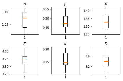
Kết quả của những suy luận của chúng tôi. Chúng tôi vẽ các giá trị maximum-likelihood cho tất cả các tham số được toàn cầu để thấy sự thay đổi của họ qua chúng tôi num_batches chạy độc lập với suy luận. Điều này tương ứng với Bảng S1 trong các tài liệu bổ sung.
fig, axs = plt.subplots(2, 3)
axs[0, 0].boxplot(best_parameters.documented_infectious_tx_rate,
                  whis=(2.5,97.5), sym='')
axs[0, 0].set_title(r'$\beta$')

axs[0, 1].boxplot(best_parameters.undocumented_infectious_tx_relative_rate,
                  whis=(2.5,97.5), sym='')
axs[0, 1].set_title(r'$\mu$')

axs[0, 2].boxplot(best_parameters.intercity_underreporting_factor,
                  whis=(2.5,97.5), sym='')
axs[0, 2].set_title(r'$\theta$')

axs[1, 0].boxplot(best_parameters.average_latency_period,
                  whis=(2.5,97.5), sym='')
axs[1, 0].set_title(r'$Z$')

axs[1, 1].boxplot(best_parameters.fraction_of_documented_infections,
                  whis=(2.5,97.5), sym='')
axs[1, 1].set_title(r'$\alpha$')

axs[1, 2].boxplot(best_parameters.average_infection_duration,
                  whis=(2.5,97.5), sym='')
axs[1, 2].set_title(r'$D$')
plt.tight_layout()