
| | |  GitHub에서 보기 GitHub에서 보기 | |
안전이 중요한 AI 응용 프로그램(예: 의료 의사 결정 및 자율 주행) 또는 데이터가 본질적으로 시끄러운 곳(예: 자연어 이해)에서는 심층 분류기가 불확실성을 안정적으로 정량화하는 것이 중요합니다. 심층 분류기는 자신의 한계와 언제 인간 전문가에게 제어권을 넘겨야 하는지 알 수 있어야 합니다. 이 튜토리얼은 SNGP (Spectral-normalized Neural Gaussian Process) 라는 기술을 사용하여 불확실성을 정량화하는 심층 분류기의 능력을 향상시키는 방법을 보여줍니다.
SNGP의 핵심 아이디어는 네트워크에 간단한 수정을 적용하여 심층 분류기의 거리 인식 을 향상시키는 것입니다. 모델의 거리 인식 은 모델의 예측 확률이 테스트 예제와 훈련 데이터 사이의 거리를 어떻게 반영하는지 측정한 것입니다. 이것은 골드 표준 확률 모델(예: RBF 커널을 사용한 가우스 프로세스 )에 일반적이지만 심층 신경망이 있는 모델에서는 부족한 바람직한 속성입니다. SNGP는 예측 정확도를 유지하면서 이 가우스 프로세스 동작을 심층 분류기에 주입하는 간단한 방법을 제공합니다.
이 튜토리얼은 두 개의 위성 데이터 세트에 대한 심층 잔차 네트워크(ResNet) 기반 SNGP 모델을 구현하고 그 불확실성 표면을 다른 두 가지 인기 있는 불확실성 접근 방식인 Monte Carlo dropout 및 Deep ensemble 의 불확실성 표면과 비교합니다.
이 튜토리얼은 장난감 2D 데이터 세트의 SNGP 모델을 보여줍니다. BERT 기반을 사용하여 실제 자연어 이해 작업에 SNGP를 적용하는 예는 SNGP-BERT 자습서 를 참조하십시오. 다양한 벤치마크 데이터 세트(예: CIFAR-100 , ImageNet , Jigsaw 독성 감지 등)에서 SNGP 모델(및 기타 여러 불확실성 방법)을 고품질로 구현하려면 Uncertainty Baselines 벤치마크를 확인하십시오.
SNGP 소개
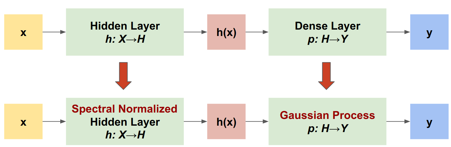
SNGP( Spectral-Normalized Neural Gaussian Process )는 유사한 수준의 정확도와 대기 시간을 유지하면서 심층 분류기의 불확실성 품질을 개선하는 간단한 접근 방식입니다. 깊은 잔여 네트워크가 주어지면 SNGP는 모델에 두 가지 간단한 변경을 수행합니다.
- 숨겨진 잔차 레이어에 스펙트럼 정규화를 적용합니다.
- 고밀도 출력 레이어를 가우시안 프로세스 레이어로 대체합니다.
다른 불확실성 접근 방식(예: Monte Carlo dropout 또는 Deep ensemble)과 비교할 때 SNGP에는 다음과 같은 몇 가지 장점이 있습니다.
- 광범위한 최신 잔차 기반 아키텍처(예: (Wide) ResNet, DenseNet, BERT 등)에서 작동합니다.
- 단일 모델 방법입니다(즉, 앙상블 평균화에 의존하지 않음). 따라서 SNGP는 단일 결정적 네트워크와 유사한 수준의 대기 시간을 가지며 ImageNet 및 Jigsaw Toxic Comments 분류 와 같은 대규모 데이터 세트로 쉽게 확장할 수 있습니다.
- 거리 인식 속성으로 인해 강력한 도메인 외부 감지 성능을 제공합니다.
이 방법의 단점은 다음과 같습니다.
SNGP의 예측 불확실성은 라플라스 근사 를 사용하여 계산됩니다. 따라서 이론적으로 SNGP의 사후 불확실성은 정확한 가우스 과정의 불확실성과 다릅니다.
SNGP 훈련은 새로운 시대를 시작할 때 공분산 재설정 단계가 필요합니다. 이것은 훈련 파이프라인에 약간의 추가 복잡성을 추가할 수 있습니다. 이 튜토리얼은 Keras 콜백을 사용하여 이것을 구현하는 간단한 방법을 보여줍니다.
설정
pip install --use-deprecated=legacy-resolver tf-models-official
# refresh pkg_resources so it takes the changes into account.
import pkg_resources
import importlib
importlib.reload(pkg_resources)
<module 'pkg_resources' from '/tmpfs/src/tf_docs_env/lib/python3.7/site-packages/pkg_resources/__init__.py'>
import matplotlib.pyplot as plt
import matplotlib.colors as colors

import sklearn.datasets

import numpy as np
import tensorflow as tf

import official.nlp.modeling.layers as nlp_layers
시각화 매크로 정의
plt.rcParams['figure.dpi'] = 140

DEFAULT_X_RANGE = (-3.5, 3.5)
DEFAULT_Y_RANGE = (-2.5, 2.5)
DEFAULT_CMAP = colors.ListedColormap(["#377eb8", "#ff7f00"])
DEFAULT_NORM = colors.Normalize(vmin=0, vmax=1,)
DEFAULT_N_GRID = 100
두 개의 달 데이터 세트
두 개의 moon 데이터 셋에서 훈련 및 평가 데이터셋을 생성합니다.
def make_training_data(sample_size=500):
  """Create two moon training dataset."""
  train_examples, train_labels = sklearn.datasets.make_moons(
      n_samples=2 * sample_size, noise=0.1)

  # Adjust data position slightly.
  train_examples[train_labels == 0] += [-0.1, 0.2]
  train_examples[train_labels == 1] += [0.1, -0.2]

  return train_examples, train_labels
전체 2D 입력 공간에서 모델의 예측 동작을 평가합니다.
def make_testing_data(x_range=DEFAULT_X_RANGE, y_range=DEFAULT_Y_RANGE, n_grid=DEFAULT_N_GRID):
  """Create a mesh grid in 2D space."""
  # testing data (mesh grid over data space)
  x = np.linspace(x_range[0], x_range[1], n_grid)
  y = np.linspace(y_range[0], y_range[1], n_grid)
  xv, yv = np.meshgrid(x, y)
  return np.stack([xv.flatten(), yv.flatten()], axis=-1)
모델 불확실성을 평가하려면 세 번째 클래스에 속하는 OOD(도메인 외) 데이터 세트를 추가하십시오. 모델은 훈련 중에 이러한 OOD 예제를 절대 볼 수 없습니다.
def make_ood_data(sample_size=500, means=(2.5, -1.75), vars=(0.01, 0.01)):
  return np.random.multivariate_normal(
      means, cov=np.diag(vars), size=sample_size)
# Load the train, test and OOD datasets.
train_examples, train_labels = make_training_data(
    sample_size=500)
test_examples = make_testing_data()
ood_examples = make_ood_data(sample_size=500)

# Visualize
pos_examples = train_examples[train_labels == 0]
neg_examples = train_examples[train_labels == 1]

plt.figure(figsize=(7, 5.5))

plt.scatter(pos_examples[:, 0], pos_examples[:, 1], c="#377eb8", alpha=0.5)
plt.scatter(neg_examples[:, 0], neg_examples[:, 1], c="#ff7f00", alpha=0.5)
plt.scatter(ood_examples[:, 0], ood_examples[:, 1], c="red", alpha=0.1)

plt.legend(["Postive", "Negative", "Out-of-Domain"])

plt.ylim(DEFAULT_Y_RANGE)
plt.xlim(DEFAULT_X_RANGE)

plt.show()

여기서 파란색과 주황색은 포지티브 및 네거티브 클래스를 나타내고 빨간색은 OOD 데이터를 나타냅니다. 불확실성을 잘 정량화하는 모델은 훈련 데이터에 가까울 때(즉, 0 또는 1에 가까운 \(p(x_{test})\) ) 확신할 것으로 예상되고, 훈련 데이터 영역에서 멀리 떨어져 있을 때(즉, 0.5에 가까운 \(p(x_{test})\) ) 불확실합니다. ).
결정론적 모델
모델 정의
(기준) 결정론적 모델에서 시작: 드롭아웃 정규화가 있는 다층 잔차 네트워크(ResNet).
class DeepResNet(tf.keras.Model):
  """Defines a multi-layer residual network."""
  def __init__(self, num_classes, num_layers=3, num_hidden=128,
               dropout_rate=0.1, **classifier_kwargs):
    super().__init__()
    # Defines class meta data.
    self.num_hidden = num_hidden
    self.num_layers = num_layers
    self.dropout_rate = dropout_rate
    self.classifier_kwargs = classifier_kwargs

    # Defines the hidden layers.
    self.input_layer = tf.keras.layers.Dense(self.num_hidden, trainable=False)
    self.dense_layers = [self.make_dense_layer() for _ in range(num_layers)]

    # Defines the output layer.
    self.classifier = self.make_output_layer(num_classes)

  def call(self, inputs):
    # Projects the 2d input data to high dimension.
    hidden = self.input_layer(inputs)

    # Computes the resnet hidden representations.
    for i in range(self.num_layers):
      resid = self.dense_layers[i](hidden)
      resid = tf.keras.layers.Dropout(self.dropout_rate)(resid)
      hidden += resid

    return self.classifier(hidden)

  def make_dense_layer(self):
    """Uses the Dense layer as the hidden layer."""
    return tf.keras.layers.Dense(self.num_hidden, activation="relu")

  def make_output_layer(self, num_classes):
    """Uses the Dense layer as the output layer."""
    return tf.keras.layers.Dense(
        num_classes, **self.classifier_kwargs)
이 튜토리얼은 128개의 은닉 유닛이 있는 6레이어 ResNet을 사용합니다.
resnet_config = dict(num_classes=2, num_layers=6, num_hidden=128)
resnet_model = DeepResNet(**resnet_config)
resnet_model.build((None, 2))
resnet_model.summary()
Model: "deep_res_net"
_________________________________________________________________
 Layer (type)                Output Shape              Param #
=================================================================
 dense (Dense)               multiple                  384

 dense_1 (Dense)             multiple                  16512

 dense_2 (Dense)             multiple                  16512

 dense_3 (Dense)             multiple                  16512

 dense_4 (Dense)             multiple                  16512

 dense_5 (Dense)             multiple                  16512

 dense_6 (Dense)             multiple                  16512

 dense_7 (Dense)             multiple                  258

=================================================================
Total params: 99,714
Trainable params: 99,330
Non-trainable params: 384
_________________________________________________________________
기차 모형
SparseCategoricalCrossentropy 를 손실 함수로 사용하고 Adam 최적화 프로그램을 사용하도록 훈련 매개변수를 구성합니다.
loss = tf.keras.losses.SparseCategoricalCrossentropy(from_logits=True)
metrics = tf.keras.metrics.SparseCategoricalAccuracy(),
optimizer = tf.keras.optimizers.Adam(learning_rate=1e-4)

train_config = dict(loss=loss, metrics=metrics, optimizer=optimizer)
배치 크기가 128인 100 Epoch에 대해 모델을 훈련시킵니다.
fit_config = dict(batch_size=128, epochs=100)
resnet_model.compile(**train_config)
resnet_model.fit(train_examples, train_labels, **fit_config)
Epoch 1/100
8/8 [==============================] - 1s 4ms/step - loss: 1.1251 - sparse_categorical_accuracy: 0.5050
Epoch 2/100
8/8 [==============================] - 0s 3ms/step - loss: 0.5538 - sparse_categorical_accuracy: 0.6920
Epoch 3/100
8/8 [==============================] - 0s 3ms/step - loss: 0.2881 - sparse_categorical_accuracy: 0.9160
Epoch 4/100
8/8 [==============================] - 0s 3ms/step - loss: 0.1923 - sparse_categorical_accuracy: 0.9370
Epoch 5/100
8/8 [==============================] - 0s 3ms/step - loss: 0.1550 - sparse_categorical_accuracy: 0.9420
Epoch 6/100
8/8 [==============================] - 0s 3ms/step - loss: 0.1403 - sparse_categorical_accuracy: 0.9450
Epoch 7/100
8/8 [==============================] - 0s 3ms/step - loss: 0.1269 - sparse_categorical_accuracy: 0.9430
Epoch 8/100
8/8 [==============================] - 0s 3ms/step - loss: 0.1208 - sparse_categorical_accuracy: 0.9460
Epoch 9/100
8/8 [==============================] - 0s 3ms/step - loss: 0.1158 - sparse_categorical_accuracy: 0.9510
Epoch 10/100
8/8 [==============================] - 0s 3ms/step - loss: 0.1103 - sparse_categorical_accuracy: 0.9490
Epoch 11/100
8/8 [==============================] - 0s 3ms/step - loss: 0.1051 - sparse_categorical_accuracy: 0.9510
Epoch 12/100
8/8 [==============================] - 0s 3ms/step - loss: 0.1053 - sparse_categorical_accuracy: 0.9510
Epoch 13/100
8/8 [==============================] - 0s 3ms/step - loss: 0.1013 - sparse_categorical_accuracy: 0.9450
Epoch 14/100
8/8 [==============================] - 0s 4ms/step - loss: 0.0967 - sparse_categorical_accuracy: 0.9500
Epoch 15/100
8/8 [==============================] - 0s 3ms/step - loss: 0.0991 - sparse_categorical_accuracy: 0.9530
Epoch 16/100
8/8 [==============================] - 0s 3ms/step - loss: 0.0984 - sparse_categorical_accuracy: 0.9500
Epoch 17/100
8/8 [==============================] - 0s 3ms/step - loss: 0.0982 - sparse_categorical_accuracy: 0.9480
Epoch 18/100
8/8 [==============================] - 0s 4ms/step - loss: 0.0918 - sparse_categorical_accuracy: 0.9510
Epoch 19/100
8/8 [==============================] - 0s 3ms/step - loss: 0.0903 - sparse_categorical_accuracy: 0.9500
Epoch 20/100
8/8 [==============================] - 0s 3ms/step - loss: 0.0883 - sparse_categorical_accuracy: 0.9510
Epoch 21/100
8/8 [==============================] - 0s 3ms/step - loss: 0.0870 - sparse_categorical_accuracy: 0.9530
Epoch 22/100
8/8 [==============================] - 0s 3ms/step - loss: 0.0884 - sparse_categorical_accuracy: 0.9560
Epoch 23/100
8/8 [==============================] - 0s 3ms/step - loss: 0.0850 - sparse_categorical_accuracy: 0.9540
Epoch 24/100
8/8 [==============================] - 0s 3ms/step - loss: 0.0808 - sparse_categorical_accuracy: 0.9580
Epoch 25/100
8/8 [==============================] - 0s 3ms/step - loss: 0.0773 - sparse_categorical_accuracy: 0.9560
Epoch 26/100
8/8 [==============================] - 0s 3ms/step - loss: 0.0801 - sparse_categorical_accuracy: 0.9590
Epoch 27/100
8/8 [==============================] - 0s 3ms/step - loss: 0.0779 - sparse_categorical_accuracy: 0.9580
Epoch 28/100
8/8 [==============================] - 0s 3ms/step - loss: 0.0807 - sparse_categorical_accuracy: 0.9580
Epoch 29/100
8/8 [==============================] - 0s 3ms/step - loss: 0.0820 - sparse_categorical_accuracy: 0.9570
Epoch 30/100
8/8 [==============================] - 0s 3ms/step - loss: 0.0730 - sparse_categorical_accuracy: 0.9600
Epoch 31/100
8/8 [==============================] - 0s 3ms/step - loss: 0.0782 - sparse_categorical_accuracy: 0.9590
Epoch 32/100
8/8 [==============================] - 0s 4ms/step - loss: 0.0704 - sparse_categorical_accuracy: 0.9600
Epoch 33/100
8/8 [==============================] - 0s 3ms/step - loss: 0.0709 - sparse_categorical_accuracy: 0.9610
Epoch 34/100
8/8 [==============================] - 0s 3ms/step - loss: 0.0758 - sparse_categorical_accuracy: 0.9580
Epoch 35/100
8/8 [==============================] - 0s 3ms/step - loss: 0.0702 - sparse_categorical_accuracy: 0.9610
Epoch 36/100
8/8 [==============================] - 0s 3ms/step - loss: 0.0688 - sparse_categorical_accuracy: 0.9600
Epoch 37/100
8/8 [==============================] - 0s 3ms/step - loss: 0.0675 - sparse_categorical_accuracy: 0.9630
Epoch 38/100
8/8 [==============================] - 0s 3ms/step - loss: 0.0636 - sparse_categorical_accuracy: 0.9690
Epoch 39/100
8/8 [==============================] - 0s 3ms/step - loss: 0.0677 - sparse_categorical_accuracy: 0.9610
Epoch 40/100
8/8 [==============================] - 0s 3ms/step - loss: 0.0702 - sparse_categorical_accuracy: 0.9650
Epoch 41/100
8/8 [==============================] - 0s 3ms/step - loss: 0.0614 - sparse_categorical_accuracy: 0.9690
Epoch 42/100
8/8 [==============================] - 0s 3ms/step - loss: 0.0663 - sparse_categorical_accuracy: 0.9680
Epoch 43/100
8/8 [==============================] - 0s 3ms/step - loss: 0.0626 - sparse_categorical_accuracy: 0.9740
Epoch 44/100
8/8 [==============================] - 0s 3ms/step - loss: 0.0590 - sparse_categorical_accuracy: 0.9760
Epoch 45/100
8/8 [==============================] - 0s 3ms/step - loss: 0.0573 - sparse_categorical_accuracy: 0.9780
Epoch 46/100
8/8 [==============================] - 0s 3ms/step - loss: 0.0568 - sparse_categorical_accuracy: 0.9770
Epoch 47/100
8/8 [==============================] - 0s 3ms/step - loss: 0.0595 - sparse_categorical_accuracy: 0.9780
Epoch 48/100
8/8 [==============================] - 0s 3ms/step - loss: 0.0482 - sparse_categorical_accuracy: 0.9840
Epoch 49/100
8/8 [==============================] - 0s 3ms/step - loss: 0.0515 - sparse_categorical_accuracy: 0.9820
Epoch 50/100
8/8 [==============================] - 0s 3ms/step - loss: 0.0525 - sparse_categorical_accuracy: 0.9830
Epoch 51/100
8/8 [==============================] - 0s 3ms/step - loss: 0.0507 - sparse_categorical_accuracy: 0.9790
Epoch 52/100
8/8 [==============================] - 0s 3ms/step - loss: 0.0433 - sparse_categorical_accuracy: 0.9850
Epoch 53/100
8/8 [==============================] - 0s 3ms/step - loss: 0.0511 - sparse_categorical_accuracy: 0.9820
Epoch 54/100
8/8 [==============================] - 0s 3ms/step - loss: 0.0501 - sparse_categorical_accuracy: 0.9820
Epoch 55/100
8/8 [==============================] - 0s 3ms/step - loss: 0.0440 - sparse_categorical_accuracy: 0.9890
Epoch 56/100
8/8 [==============================] - 0s 3ms/step - loss: 0.0438 - sparse_categorical_accuracy: 0.9850
Epoch 57/100
8/8 [==============================] - 0s 3ms/step - loss: 0.0438 - sparse_categorical_accuracy: 0.9880
Epoch 58/100
8/8 [==============================] - 0s 3ms/step - loss: 0.0416 - sparse_categorical_accuracy: 0.9860
Epoch 59/100
8/8 [==============================] - 0s 3ms/step - loss: 0.0479 - sparse_categorical_accuracy: 0.9860
Epoch 60/100
8/8 [==============================] - 0s 3ms/step - loss: 0.0434 - sparse_categorical_accuracy: 0.9860
Epoch 61/100
8/8 [==============================] - 0s 3ms/step - loss: 0.0414 - sparse_categorical_accuracy: 0.9880
Epoch 62/100
8/8 [==============================] - 0s 3ms/step - loss: 0.0402 - sparse_categorical_accuracy: 0.9870
Epoch 63/100
8/8 [==============================] - 0s 3ms/step - loss: 0.0376 - sparse_categorical_accuracy: 0.9890
Epoch 64/100
8/8 [==============================] - 0s 3ms/step - loss: 0.0337 - sparse_categorical_accuracy: 0.9900
Epoch 65/100
8/8 [==============================] - 0s 3ms/step - loss: 0.0309 - sparse_categorical_accuracy: 0.9910
Epoch 66/100
8/8 [==============================] - 0s 3ms/step - loss: 0.0336 - sparse_categorical_accuracy: 0.9910
Epoch 67/100
8/8 [==============================] - 0s 3ms/step - loss: 0.0389 - sparse_categorical_accuracy: 0.9870
Epoch 68/100
8/8 [==============================] - 0s 3ms/step - loss: 0.0333 - sparse_categorical_accuracy: 0.9920
Epoch 69/100
8/8 [==============================] - 0s 3ms/step - loss: 0.0331 - sparse_categorical_accuracy: 0.9890
Epoch 70/100
8/8 [==============================] - 0s 3ms/step - loss: 0.0346 - sparse_categorical_accuracy: 0.9900
Epoch 71/100
8/8 [==============================] - 0s 3ms/step - loss: 0.0367 - sparse_categorical_accuracy: 0.9880
Epoch 72/100
8/8 [==============================] - 0s 3ms/step - loss: 0.0283 - sparse_categorical_accuracy: 0.9920
Epoch 73/100
8/8 [==============================] - 0s 3ms/step - loss: 0.0315 - sparse_categorical_accuracy: 0.9930
Epoch 74/100
8/8 [==============================] - 0s 3ms/step - loss: 0.0271 - sparse_categorical_accuracy: 0.9900
Epoch 75/100
8/8 [==============================] - 0s 3ms/step - loss: 0.0257 - sparse_categorical_accuracy: 0.9920
Epoch 76/100
8/8 [==============================] - 0s 3ms/step - loss: 0.0289 - sparse_categorical_accuracy: 0.9900
Epoch 77/100
8/8 [==============================] - 0s 3ms/step - loss: 0.0264 - sparse_categorical_accuracy: 0.9900
Epoch 78/100
8/8 [==============================] - 0s 3ms/step - loss: 0.0272 - sparse_categorical_accuracy: 0.9910
Epoch 79/100
8/8 [==============================] - 0s 3ms/step - loss: 0.0336 - sparse_categorical_accuracy: 0.9880
Epoch 80/100
8/8 [==============================] - 0s 3ms/step - loss: 0.0249 - sparse_categorical_accuracy: 0.9900
Epoch 81/100
8/8 [==============================] - 0s 3ms/step - loss: 0.0216 - sparse_categorical_accuracy: 0.9930
Epoch 82/100
8/8 [==============================] - 0s 3ms/step - loss: 0.0279 - sparse_categorical_accuracy: 0.9890
Epoch 83/100
8/8 [==============================] - 0s 3ms/step - loss: 0.0261 - sparse_categorical_accuracy: 0.9920
Epoch 84/100
8/8 [==============================] - 0s 3ms/step - loss: 0.0235 - sparse_categorical_accuracy: 0.9920
Epoch 85/100
8/8 [==============================] - 0s 3ms/step - loss: 0.0236 - sparse_categorical_accuracy: 0.9930
Epoch 86/100
8/8 [==============================] - 0s 3ms/step - loss: 0.0219 - sparse_categorical_accuracy: 0.9920
Epoch 87/100
8/8 [==============================] - 0s 3ms/step - loss: 0.0196 - sparse_categorical_accuracy: 0.9920
Epoch 88/100
8/8 [==============================] - 0s 3ms/step - loss: 0.0215 - sparse_categorical_accuracy: 0.9900
Epoch 89/100
8/8 [==============================] - 0s 3ms/step - loss: 0.0223 - sparse_categorical_accuracy: 0.9900
Epoch 90/100
8/8 [==============================] - 0s 3ms/step - loss: 0.0200 - sparse_categorical_accuracy: 0.9950
Epoch 91/100
8/8 [==============================] - 0s 3ms/step - loss: 0.0250 - sparse_categorical_accuracy: 0.9900
Epoch 92/100
8/8 [==============================] - 0s 3ms/step - loss: 0.0160 - sparse_categorical_accuracy: 0.9940
Epoch 93/100
8/8 [==============================] - 0s 3ms/step - loss: 0.0203 - sparse_categorical_accuracy: 0.9930
Epoch 94/100
8/8 [==============================] - 0s 3ms/step - loss: 0.0203 - sparse_categorical_accuracy: 0.9930
Epoch 95/100
8/8 [==============================] - 0s 3ms/step - loss: 0.0172 - sparse_categorical_accuracy: 0.9960
Epoch 96/100
8/8 [==============================] - 0s 3ms/step - loss: 0.0209 - sparse_categorical_accuracy: 0.9940
Epoch 97/100
8/8 [==============================] - 0s 3ms/step - loss: 0.0179 - sparse_categorical_accuracy: 0.9920
Epoch 98/100
8/8 [==============================] - 0s 3ms/step - loss: 0.0195 - sparse_categorical_accuracy: 0.9940
Epoch 99/100
8/8 [==============================] - 0s 3ms/step - loss: 0.0165 - sparse_categorical_accuracy: 0.9930
Epoch 100/100
8/8 [==============================] - 0s 3ms/step - loss: 0.0170 - sparse_categorical_accuracy: 0.9950
<keras.callbacks.History at 0x7ff7ac5c8fd0>
불확실성 시각화
def plot_uncertainty_surface(test_uncertainty, ax, cmap=None):
  """Visualizes the 2D uncertainty surface.

  For simplicity, assume these objects already exist in the memory:

    test_examples: Array of test examples, shape (num_test, 2).
    train_labels: Array of train labels, shape (num_train, ).
    train_examples: Array of train examples, shape (num_train, 2).

  Arguments:
    test_uncertainty: Array of uncertainty scores, shape (num_test,).
    ax: A matplotlib Axes object that specifies a matplotlib figure.
    cmap: A matplotlib colormap object specifying the palette of the
      predictive surface.

  Returns:
    pcm: A matplotlib PathCollection object that contains the palette
      information of the uncertainty plot.
  """
  # Normalize uncertainty for better visualization.
  test_uncertainty = test_uncertainty / np.max(test_uncertainty)

  # Set view limits.
  ax.set_ylim(DEFAULT_Y_RANGE)
  ax.set_xlim(DEFAULT_X_RANGE)

  # Plot normalized uncertainty surface.
  pcm = ax.imshow(
      np.reshape(test_uncertainty, [DEFAULT_N_GRID, DEFAULT_N_GRID]),
      cmap=cmap,
      origin="lower",
      extent=DEFAULT_X_RANGE + DEFAULT_Y_RANGE,
      vmin=DEFAULT_NORM.vmin,
      vmax=DEFAULT_NORM.vmax,
      interpolation='bicubic',
      aspect='auto')

  # Plot training data.
  ax.scatter(train_examples[:, 0], train_examples[:, 1],
             c=train_labels, cmap=DEFAULT_CMAP, alpha=0.5)
  ax.scatter(ood_examples[:, 0], ood_examples[:, 1], c="red", alpha=0.1)

  return pcm
이제 결정론적 모델의 예측을 시각화합니다. 먼저 클래스 확률을 플로팅합니다.
\[p(x) = softmax(logit(x))\]
resnet_logits = resnet_model(test_examples)
resnet_probs = tf.nn.softmax(resnet_logits, axis=-1)[:, 0]  # Take the probability for class 0.
_, ax = plt.subplots(figsize=(7, 5.5))

pcm = plot_uncertainty_surface(resnet_probs, ax=ax)

plt.colorbar(pcm, ax=ax)
plt.title("Class Probability, Deterministic Model")

plt.show()

이 그림에서 노란색과 보라색은 두 클래스에 대한 예측 확률입니다. 결정론적 모델은 두 개의 알려진 클래스(파란색 및 주황색)를 비선형 결정 경계로 분류하는 데 좋은 작업을 수행했습니다. 그러나 거리 인식 이 되지 않고, 한번도 본 적 없는 빨간색 OOD(out-of-domain) 사례를 주황색 클래스로 자신 있게 분류했습니다.
예측 분산 을 계산하여 모델 불확실성을 시각화합니다.
\[var(x) = p(x) * (1 - p(x))\]
resnet_uncertainty = resnet_probs * (1 - resnet_probs)
_, ax = plt.subplots(figsize=(7, 5.5))

pcm = plot_uncertainty_surface(resnet_uncertainty, ax=ax)

plt.colorbar(pcm, ax=ax)
plt.title("Predictive Uncertainty, Deterministic Model")

plt.show()

이 그림에서 노란색은 높은 불확실성을 나타내고 보라색은 낮은 불확실성을 나타냅니다. 결정적 ResNet의 불확실성은 결정 경계에서 테스트 예제의 거리에만 의존합니다. 이것은 모델이 훈련 도메인을 벗어날 때 지나치게 자신감 있게 만듭니다. 다음 섹션에서는 SNGP가 이 데이터 세트에서 어떻게 다르게 작동하는지 보여줍니다.
SNGP 모델
SNGP 모델 정의
이제 SNGP 모델을 구현해 보겠습니다. SNGP 구성 요소인 SpectralNormalization 및 RandomFeatureGaussianProcess 모두 tensorflow_model의 내장 레이어에서 사용할 수 있습니다.
이 두 가지 구성 요소를 더 자세히 살펴보겠습니다. ( SNGP 모델 섹션으로 이동하여 전체 모델이 구현되는 방식을 확인할 수도 있습니다.)
스펙트럼 정규화 래퍼
SpectralNormalization 은 Keras 레이어 래퍼입니다. 다음과 같이 기존 Dense 레이어에 적용할 수 있습니다.
dense = tf.keras.layers.Dense(units=10)
dense = nlp_layers.SpectralNormalization(dense, norm_multiplier=0.9)
스펙트럼 정규화는 스펙트럼 노름(즉, \(W\)의 가장 큰 고유값)을 대상 값 norm_multiplier 로 점진적으로 안내하여 숨겨진 가중치 \(W\) 를 정규화합니다.
가우스 프로세스(GP) 계층
RandomFeatureGaussianProcess 는 심층 신경망으로 종단 간 학습이 가능한 가우스 프로세스 모델에 대한 임의 기능 기반 근사 를 구현합니다. 내부적으로 Gaussian 프로세스 계층은 2계층 네트워크를 구현합니다.
\[logits(x) = \Phi(x) \beta, \quad \Phi(x)=\sqrt{\frac{2}{M} } * cos(Wx + b)\]
여기서 \(x\) 은 입력이고 \(W\) 와 \(b\) 은 각각 가우스 분포와 균일 분포에서 무작위로 초기화된 고정 가중치입니다. (따라서 \(\Phi(x)\) 을 "random feature"라고 합니다.) \(\beta\) 는 Dense 레이어와 유사한 학습 가능한 커널 가중치입니다.
batch_size = 32
input_dim = 1024
num_classes = 10
gp_layer = nlp_layers.RandomFeatureGaussianProcess(units=num_classes,
                                               num_inducing=1024,
                                               normalize_input=False,
                                               scale_random_features=True,
                                               gp_cov_momentum=-1)
GP 레이어의 주요 매개변수는 다음과 같습니다.
-
units: 출력 로짓의 차원입니다. -
num_inducing: 은닉 가중치 \(W\) \(M\) -placeholder13 . 기본값은 1024입니다. -
normalize_input: 레이어 정규화를 입력 \(x\)에 적용할지 여부입니다. -
scale_random_features: \(\sqrt{2/M}\) 스케일을 숨겨진 출력에 적용할지 여부입니다.
-
gp_cov_momentum은 모델 공분산이 계산되는 방법을 제어합니다. 양수 값(예: 0.999)으로 설정하면 공분산 행렬은 운동량 기반 이동 평균 업데이트(배치 정규화와 유사)를 사용하여 계산됩니다. -1로 설정하면 공분산 행렬이 운동량 없이 업데이트됩니다.
모양이 (batch_size, input_dim) 인 배치 입력이 주어지면 GP 계층은 예측을 위해 logits 텐서(shape (batch_size, num_classes) )와 의 사후 공분산 행렬인 covmat 텐서(shape (batch_size, batch_size) )를 반환합니다. 배치 로지츠.
embedding = tf.random.normal(shape=(batch_size, input_dim))

logits, covmat = gp_layer(embedding)
이론적으로 알고리즘을 확장하여 서로 다른 클래스에 대해 서로 다른 분산 값을 계산할 수 있습니다( 원본 SNGP 문서 에서 소개됨). 그러나 이것은 큰 출력 공간(예: ImageNet 또는 언어 모델링)의 문제로 확장하기 어렵습니다.
전체 SNGP 모델
기본 클래스 DeepResNet 이 주어지면 SNGP 모델은 잔차 네트워크의 은닉 및 출력 레이어를 수정하여 쉽게 구현할 수 있습니다. model.fit() API와의 호환성을 위해 모델의 call() 메서드도 수정하여 훈련 중에 logits 만 출력하도록 합니다.
class DeepResNetSNGP(DeepResNet):
  def __init__(self, spec_norm_bound=0.9, **kwargs):
    self.spec_norm_bound = spec_norm_bound
    super().__init__(**kwargs)

  def make_dense_layer(self):
    """Applies spectral normalization to the hidden layer."""
    dense_layer = super().make_dense_layer()
    return nlp_layers.SpectralNormalization(
        dense_layer, norm_multiplier=self.spec_norm_bound)

  def make_output_layer(self, num_classes):
    """Uses Gaussian process as the output layer."""
    return nlp_layers.RandomFeatureGaussianProcess(
        num_classes,
        gp_cov_momentum=-1,
        **self.classifier_kwargs)

  def call(self, inputs, training=False, return_covmat=False):
    # Gets logits and covariance matrix from GP layer.
    logits, covmat = super().call(inputs)

    # Returns only logits during training.
    if not training and return_covmat:
      return logits, covmat

    return logits
결정적 모델과 동일한 아키텍처를 사용합니다.
resnet_config
{'num_classes': 2, 'num_layers': 6, 'num_hidden': 128}
sngp_model = DeepResNetSNGP(**resnet_config)
sngp_model.build((None, 2))
sngp_model.summary()
Model: "deep_res_net_sngp"
_________________________________________________________________
 Layer (type)                Output Shape              Param #
=================================================================
 dense_9 (Dense)             multiple                  384

 spectral_normalization_1 (S  multiple                 16768
 pectralNormalization)

 spectral_normalization_2 (S  multiple                 16768
 pectralNormalization)

 spectral_normalization_3 (S  multiple                 16768
 pectralNormalization)

 spectral_normalization_4 (S  multiple                 16768
 pectralNormalization)

 spectral_normalization_5 (S  multiple                 16768
 pectralNormalization)

 spectral_normalization_6 (S  multiple                 16768
 pectralNormalization)

 random_feature_gaussian_pro  multiple                 1182722
 cess (RandomFeatureGaussian
 Process)

=================================================================
Total params: 1,283,714
Trainable params: 101,120
Non-trainable params: 1,182,594
_________________________________________________________________
새 에포크가 시작될 때 공분산 행렬을 재설정하기 위해 Keras 콜백을 구현합니다.
class ResetCovarianceCallback(tf.keras.callbacks.Callback):

  def on_epoch_begin(self, epoch, logs=None):
    """Resets covariance matrix at the begining of the epoch."""
    if epoch > 0:
      self.model.classifier.reset_covariance_matrix()
이 콜백을 DeepResNetSNGP 모델 클래스에 추가하십시오.
class DeepResNetSNGPWithCovReset(DeepResNetSNGP):
  def fit(self, *args, **kwargs):
    """Adds ResetCovarianceCallback to model callbacks."""
    kwargs["callbacks"] = list(kwargs.get("callbacks", []))
    kwargs["callbacks"].append(ResetCovarianceCallback())

    return super().fit(*args, **kwargs)
기차 모형
tf.keras.model.fit 을 사용하여 모델을 훈련시키십시오.
sngp_model = DeepResNetSNGPWithCovReset(**resnet_config)
sngp_model.compile(**train_config)
sngp_model.fit(train_examples, train_labels, **fit_config)
Epoch 1/100
8/8 [==============================] - 2s 5ms/step - loss: 0.6223 - sparse_categorical_accuracy: 0.9570
Epoch 2/100
8/8 [==============================] - 0s 4ms/step - loss: 0.5310 - sparse_categorical_accuracy: 0.9980
Epoch 3/100
8/8 [==============================] - 0s 4ms/step - loss: 0.4766 - sparse_categorical_accuracy: 0.9990
Epoch 4/100
8/8 [==============================] - 0s 5ms/step - loss: 0.4346 - sparse_categorical_accuracy: 0.9980
Epoch 5/100
8/8 [==============================] - 0s 5ms/step - loss: 0.4015 - sparse_categorical_accuracy: 0.9980
Epoch 6/100
8/8 [==============================] - 0s 5ms/step - loss: 0.3757 - sparse_categorical_accuracy: 0.9990
Epoch 7/100
8/8 [==============================] - 0s 4ms/step - loss: 0.3525 - sparse_categorical_accuracy: 0.9990
Epoch 8/100
8/8 [==============================] - 0s 4ms/step - loss: 0.3305 - sparse_categorical_accuracy: 0.9990
Epoch 9/100
8/8 [==============================] - 0s 5ms/step - loss: 0.3144 - sparse_categorical_accuracy: 0.9980
Epoch 10/100
8/8 [==============================] - 0s 5ms/step - loss: 0.2975 - sparse_categorical_accuracy: 0.9990
Epoch 11/100
8/8 [==============================] - 0s 4ms/step - loss: 0.2832 - sparse_categorical_accuracy: 0.9990
Epoch 12/100
8/8 [==============================] - 0s 5ms/step - loss: 0.2707 - sparse_categorical_accuracy: 0.9990
Epoch 13/100
8/8 [==============================] - 0s 4ms/step - loss: 0.2568 - sparse_categorical_accuracy: 0.9990
Epoch 14/100
8/8 [==============================] - 0s 4ms/step - loss: 0.2470 - sparse_categorical_accuracy: 0.9970
Epoch 15/100
8/8 [==============================] - 0s 4ms/step - loss: 0.2361 - sparse_categorical_accuracy: 0.9990
Epoch 16/100
8/8 [==============================] - 0s 5ms/step - loss: 0.2271 - sparse_categorical_accuracy: 0.9990
Epoch 17/100
8/8 [==============================] - 0s 5ms/step - loss: 0.2182 - sparse_categorical_accuracy: 0.9990
Epoch 18/100
8/8 [==============================] - 0s 4ms/step - loss: 0.2097 - sparse_categorical_accuracy: 0.9990
Epoch 19/100
8/8 [==============================] - 0s 4ms/step - loss: 0.2018 - sparse_categorical_accuracy: 0.9990
Epoch 20/100
8/8 [==============================] - 0s 4ms/step - loss: 0.1940 - sparse_categorical_accuracy: 0.9980
Epoch 21/100
8/8 [==============================] - 0s 4ms/step - loss: 0.1892 - sparse_categorical_accuracy: 0.9990
Epoch 22/100
8/8 [==============================] - 0s 4ms/step - loss: 0.1821 - sparse_categorical_accuracy: 0.9980
Epoch 23/100
8/8 [==============================] - 0s 4ms/step - loss: 0.1768 - sparse_categorical_accuracy: 0.9990
Epoch 24/100
8/8 [==============================] - 0s 4ms/step - loss: 0.1702 - sparse_categorical_accuracy: 0.9980
Epoch 25/100
8/8 [==============================] - 0s 4ms/step - loss: 0.1664 - sparse_categorical_accuracy: 0.9990
Epoch 26/100
8/8 [==============================] - 0s 4ms/step - loss: 0.1604 - sparse_categorical_accuracy: 0.9990
Epoch 27/100
8/8 [==============================] - 0s 4ms/step - loss: 0.1565 - sparse_categorical_accuracy: 0.9990
Epoch 28/100
8/8 [==============================] - 0s 4ms/step - loss: 0.1517 - sparse_categorical_accuracy: 0.9990
Epoch 29/100
8/8 [==============================] - 0s 4ms/step - loss: 0.1469 - sparse_categorical_accuracy: 0.9990
Epoch 30/100
8/8 [==============================] - 0s 4ms/step - loss: 0.1431 - sparse_categorical_accuracy: 0.9980
Epoch 31/100
8/8 [==============================] - 0s 4ms/step - loss: 0.1385 - sparse_categorical_accuracy: 0.9980
Epoch 32/100
8/8 [==============================] - 0s 4ms/step - loss: 0.1351 - sparse_categorical_accuracy: 0.9990
Epoch 33/100
8/8 [==============================] - 0s 5ms/step - loss: 0.1312 - sparse_categorical_accuracy: 0.9980
Epoch 34/100
8/8 [==============================] - 0s 4ms/step - loss: 0.1289 - sparse_categorical_accuracy: 0.9990
Epoch 35/100
8/8 [==============================] - 0s 4ms/step - loss: 0.1254 - sparse_categorical_accuracy: 0.9980
Epoch 36/100
8/8 [==============================] - 0s 4ms/step - loss: 0.1223 - sparse_categorical_accuracy: 0.9980
Epoch 37/100
8/8 [==============================] - 0s 4ms/step - loss: 0.1180 - sparse_categorical_accuracy: 0.9990
Epoch 38/100
8/8 [==============================] - 0s 4ms/step - loss: 0.1167 - sparse_categorical_accuracy: 0.9990
Epoch 39/100
8/8 [==============================] - 0s 4ms/step - loss: 0.1132 - sparse_categorical_accuracy: 0.9980
Epoch 40/100
8/8 [==============================] - 0s 4ms/step - loss: 0.1110 - sparse_categorical_accuracy: 0.9990
Epoch 41/100
8/8 [==============================] - 0s 4ms/step - loss: 0.1075 - sparse_categorical_accuracy: 0.9990
Epoch 42/100
8/8 [==============================] - 0s 4ms/step - loss: 0.1067 - sparse_categorical_accuracy: 0.9990
Epoch 43/100
8/8 [==============================] - 0s 4ms/step - loss: 0.1034 - sparse_categorical_accuracy: 0.9990
Epoch 44/100
8/8 [==============================] - 0s 4ms/step - loss: 0.1006 - sparse_categorical_accuracy: 0.9990
Epoch 45/100
8/8 [==============================] - 0s 5ms/step - loss: 0.0991 - sparse_categorical_accuracy: 0.9990
Epoch 46/100
8/8 [==============================] - 0s 5ms/step - loss: 0.0963 - sparse_categorical_accuracy: 0.9990
Epoch 47/100
8/8 [==============================] - 0s 5ms/step - loss: 0.0943 - sparse_categorical_accuracy: 0.9980
Epoch 48/100
8/8 [==============================] - 0s 5ms/step - loss: 0.0925 - sparse_categorical_accuracy: 0.9990
Epoch 49/100
8/8 [==============================] - 0s 4ms/step - loss: 0.0905 - sparse_categorical_accuracy: 0.9990
Epoch 50/100
8/8 [==============================] - 0s 5ms/step - loss: 0.0889 - sparse_categorical_accuracy: 0.9990
Epoch 51/100
8/8 [==============================] - 0s 5ms/step - loss: 0.0863 - sparse_categorical_accuracy: 0.9980
Epoch 52/100
8/8 [==============================] - 0s 5ms/step - loss: 0.0847 - sparse_categorical_accuracy: 0.9990
Epoch 53/100
8/8 [==============================] - 0s 5ms/step - loss: 0.0831 - sparse_categorical_accuracy: 0.9980
Epoch 54/100
8/8 [==============================] - 0s 5ms/step - loss: 0.0818 - sparse_categorical_accuracy: 0.9990
Epoch 55/100
8/8 [==============================] - 0s 5ms/step - loss: 0.0799 - sparse_categorical_accuracy: 0.9990
Epoch 56/100
8/8 [==============================] - 0s 4ms/step - loss: 0.0780 - sparse_categorical_accuracy: 0.9990
Epoch 57/100
8/8 [==============================] - 0s 5ms/step - loss: 0.0768 - sparse_categorical_accuracy: 0.9990
Epoch 58/100
8/8 [==============================] - 0s 4ms/step - loss: 0.0751 - sparse_categorical_accuracy: 0.9990
Epoch 59/100
8/8 [==============================] - 0s 4ms/step - loss: 0.0748 - sparse_categorical_accuracy: 0.9990
Epoch 60/100
8/8 [==============================] - 0s 4ms/step - loss: 0.0723 - sparse_categorical_accuracy: 0.9990
Epoch 61/100
8/8 [==============================] - 0s 4ms/step - loss: 0.0712 - sparse_categorical_accuracy: 0.9990
Epoch 62/100
8/8 [==============================] - 0s 4ms/step - loss: 0.0701 - sparse_categorical_accuracy: 0.9990
Epoch 63/100
8/8 [==============================] - 0s 4ms/step - loss: 0.0701 - sparse_categorical_accuracy: 0.9990
Epoch 64/100
8/8 [==============================] - 0s 4ms/step - loss: 0.0683 - sparse_categorical_accuracy: 0.9990
Epoch 65/100
8/8 [==============================] - 0s 5ms/step - loss: 0.0665 - sparse_categorical_accuracy: 0.9990
Epoch 66/100
8/8 [==============================] - 0s 5ms/step - loss: 0.0661 - sparse_categorical_accuracy: 0.9990
Epoch 67/100
8/8 [==============================] - 0s 5ms/step - loss: 0.0636 - sparse_categorical_accuracy: 0.9990
Epoch 68/100
8/8 [==============================] - 0s 4ms/step - loss: 0.0631 - sparse_categorical_accuracy: 0.9990
Epoch 69/100
8/8 [==============================] - 0s 4ms/step - loss: 0.0620 - sparse_categorical_accuracy: 0.9990
Epoch 70/100
8/8 [==============================] - 0s 5ms/step - loss: 0.0606 - sparse_categorical_accuracy: 0.9990
Epoch 71/100
8/8 [==============================] - 0s 4ms/step - loss: 0.0601 - sparse_categorical_accuracy: 0.9980
Epoch 72/100
8/8 [==============================] - 0s 4ms/step - loss: 0.0590 - sparse_categorical_accuracy: 0.9990
Epoch 73/100
8/8 [==============================] - 0s 4ms/step - loss: 0.0586 - sparse_categorical_accuracy: 0.9990
Epoch 74/100
8/8 [==============================] - 0s 4ms/step - loss: 0.0574 - sparse_categorical_accuracy: 0.9990
Epoch 75/100
8/8 [==============================] - 0s 4ms/step - loss: 0.0565 - sparse_categorical_accuracy: 1.0000
Epoch 76/100
8/8 [==============================] - 0s 4ms/step - loss: 0.0559 - sparse_categorical_accuracy: 0.9990
Epoch 77/100
8/8 [==============================] - 0s 4ms/step - loss: 0.0549 - sparse_categorical_accuracy: 0.9990
Epoch 78/100
8/8 [==============================] - 0s 5ms/step - loss: 0.0534 - sparse_categorical_accuracy: 1.0000
Epoch 79/100
8/8 [==============================] - 0s 5ms/step - loss: 0.0532 - sparse_categorical_accuracy: 0.9990
Epoch 80/100
8/8 [==============================] - 0s 4ms/step - loss: 0.0519 - sparse_categorical_accuracy: 1.0000
Epoch 81/100
8/8 [==============================] - 0s 4ms/step - loss: 0.0511 - sparse_categorical_accuracy: 1.0000
Epoch 82/100
8/8 [==============================] - 0s 4ms/step - loss: 0.0508 - sparse_categorical_accuracy: 0.9990
Epoch 83/100
8/8 [==============================] - 0s 4ms/step - loss: 0.0499 - sparse_categorical_accuracy: 1.0000
Epoch 84/100
8/8 [==============================] - 0s 4ms/step - loss: 0.0490 - sparse_categorical_accuracy: 1.0000
Epoch 85/100
8/8 [==============================] - 0s 4ms/step - loss: 0.0490 - sparse_categorical_accuracy: 0.9990
Epoch 86/100
8/8 [==============================] - 0s 5ms/step - loss: 0.0470 - sparse_categorical_accuracy: 1.0000
Epoch 87/100
8/8 [==============================] - 0s 4ms/step - loss: 0.0468 - sparse_categorical_accuracy: 1.0000
Epoch 88/100
8/8 [==============================] - 0s 4ms/step - loss: 0.0468 - sparse_categorical_accuracy: 1.0000
Epoch 89/100
8/8 [==============================] - 0s 4ms/step - loss: 0.0453 - sparse_categorical_accuracy: 1.0000
Epoch 90/100
8/8 [==============================] - 0s 4ms/step - loss: 0.0448 - sparse_categorical_accuracy: 1.0000
Epoch 91/100
8/8 [==============================] - 0s 4ms/step - loss: 0.0441 - sparse_categorical_accuracy: 1.0000
Epoch 92/100
8/8 [==============================] - 0s 4ms/step - loss: 0.0434 - sparse_categorical_accuracy: 1.0000
Epoch 93/100
8/8 [==============================] - 0s 5ms/step - loss: 0.0431 - sparse_categorical_accuracy: 1.0000
Epoch 94/100
8/8 [==============================] - 0s 5ms/step - loss: 0.0424 - sparse_categorical_accuracy: 1.0000
Epoch 95/100
8/8 [==============================] - 0s 5ms/step - loss: 0.0420 - sparse_categorical_accuracy: 1.0000
Epoch 96/100
8/8 [==============================] - 0s 4ms/step - loss: 0.0415 - sparse_categorical_accuracy: 1.0000
Epoch 97/100
8/8 [==============================] - 0s 4ms/step - loss: 0.0409 - sparse_categorical_accuracy: 1.0000
Epoch 98/100
8/8 [==============================] - 0s 4ms/step - loss: 0.0401 - sparse_categorical_accuracy: 1.0000
Epoch 99/100
8/8 [==============================] - 0s 5ms/step - loss: 0.0396 - sparse_categorical_accuracy: 1.0000
Epoch 100/100
8/8 [==============================] - 0s 5ms/step - loss: 0.0392 - sparse_categorical_accuracy: 1.0000
<keras.callbacks.History at 0x7ff7ac0f83d0>
불확실성 시각화
먼저 예측 로짓과 분산을 계산합니다.
sngp_logits, sngp_covmat = sngp_model(test_examples, return_covmat=True)
sngp_variance = tf.linalg.diag_part(sngp_covmat)[:, None]
이제 사후 예측 확률을 계산합니다. 확률 모델의 예측 확률을 계산하는 고전적인 방법은 몬테카를로 샘플링을 사용하는 것입니다. 즉,
\[E(p(x)) = \frac{1}{M} \sum_{m=1}^M logit_m(x), \]
여기서 \(M\) 은 샘플 크기이고 \(logit_m(x)\) 는 SNGP 사후 \(MultivariateNormal\)( sngp_logits , sngp_covmat )의 무작위 샘플입니다. 그러나 이 접근 방식은 자율 주행이나 실시간 입찰과 같이 지연 시간에 민감한 애플리케이션의 경우 느릴 수 있습니다. 대신 mean-field 방법 을 사용하여 \(E(p(x))\) 를 근사할 수 있습니다.
\[E(p(x)) \approx softmax(\frac{logit(x)}{\sqrt{1+ \lambda * \sigma^2(x)} })\]
여기서 \(\sigma^2(x)\) 은 SNGP 분산이고 \(\lambda\) 은 종종 \(\pi/8\) 또는 \(3/\pi^2\)로 선택됩니다.
sngp_logits_adjusted = sngp_logits / tf.sqrt(1. + (np.pi / 8.) * sngp_variance)
sngp_probs = tf.nn.softmax(sngp_logits_adjusted, axis=-1)[:, 0]
이 평균 필드 방법은 내장 함수 layers.gaussian_process.mean_field_logits 로 구현됩니다.
def compute_posterior_mean_probability(logits, covmat, lambda_param=np.pi / 8.):
  # Computes uncertainty-adjusted logits using the built-in method.
  logits_adjusted = nlp_layers.gaussian_process.mean_field_logits(
      logits, covmat, mean_field_factor=lambda_param)

  return tf.nn.softmax(logits_adjusted, axis=-1)[:, 0]
sngp_logits, sngp_covmat = sngp_model(test_examples, return_covmat=True)
sngp_probs = compute_posterior_mean_probability(sngp_logits, sngp_covmat)
SNGP 요약
def plot_predictions(pred_probs, model_name=""):
  """Plot normalized class probabilities and predictive uncertainties."""
  # Compute predictive uncertainty.
  uncertainty = pred_probs * (1. - pred_probs)

  # Initialize the plot axes.
  fig, axs = plt.subplots(1, 2, figsize=(14, 5))

  # Plots the class probability.
  pcm_0 = plot_uncertainty_surface(pred_probs, ax=axs[0])
  # Plots the predictive uncertainty.
  pcm_1 = plot_uncertainty_surface(uncertainty, ax=axs[1])

  # Adds color bars and titles.
  fig.colorbar(pcm_0, ax=axs[0])
  fig.colorbar(pcm_1, ax=axs[1])

  axs[0].set_title(f"Class Probability, {model_name}")
  axs[1].set_title(f"(Normalized) Predictive Uncertainty, {model_name}")

  plt.show()
모든 것을 함께하십시오. 전체 절차(훈련, 평가 및 불확실성 계산)는 단 5줄로 수행할 수 있습니다.
def train_and_test_sngp(train_examples, test_examples):
  sngp_model = DeepResNetSNGPWithCovReset(**resnet_config)

  sngp_model.compile(**train_config)
  sngp_model.fit(train_examples, train_labels, verbose=0, **fit_config)

  sngp_logits, sngp_covmat = sngp_model(test_examples, return_covmat=True)
  sngp_probs = compute_posterior_mean_probability(sngp_logits, sngp_covmat)

  return sngp_probs
sngp_probs = train_and_test_sngp(train_examples, test_examples)
SNGP 모델의 클래스 확률(왼쪽)과 예측 불확실성(오른쪽)을 시각화합니다.
plot_predictions(sngp_probs, model_name="SNGP")

클래스 확률 플롯(왼쪽)에서 노란색과 보라색은 클래스 확률임을 기억하십시오. 훈련 데이터 도메인에 가까울 때 SNGP는 높은 신뢰도로 예를 올바르게 분류합니다(즉, 0 또는 1에 가까운 확률 할당). 훈련 데이터에서 멀어지면 SNGP는 점차 자신감이 떨어지고 예측 확률은 0.5에 가까워지는 반면 (정규화된) 모델 불확실성은 1로 올라갑니다.
이것을 결정론적 모델의 불확실성 표면과 비교하십시오.
plot_predictions(resnet_probs, model_name="Deterministic")

앞서 언급했듯이 결정론적 모델은 거리를 인식 하지 않습니다. 불확실성은 결정 경계에서 테스트 예제의 거리로 정의됩니다. 이로 인해 모델이 도메인 외부 예제(빨간색)에 대해 과신 예측을 생성합니다.
다른 불확실성 접근법과의 비교
이 섹션에서는 SNGP의 불확실성을 Monte Carlo dropout 및 Deep ensemble 과 비교합니다.
이 두 가지 방법 모두 결정론적 모델의 다중 전진 패스의 Monte Carlo 평균을 기반으로 합니다. 먼저 앙상블 크기 \(M\)설정합니다.
num_ensemble = 10
몬테카를로 탈락
Dropout 레이어가 있는 훈련된 신경망이 주어지면 Monte Carlo dropout 은 평균 예측 확률을 계산합니다.
\[E(p(x)) = \frac{1}{M}\sum_{m=1}^M softmax(logit_m(x))\]
여러 Dropout 지원 정방향 패스 \(\{logit_m(x)\}_{m=1}^M\)에 대한 평균을 구합니다.
def mc_dropout_sampling(test_examples):
  # Enable dropout during inference.
  return resnet_model(test_examples, training=True)
# Monte Carlo dropout inference.
dropout_logit_samples = [mc_dropout_sampling(test_examples) for _ in range(num_ensemble)]
dropout_prob_samples = [tf.nn.softmax(dropout_logits, axis=-1)[:, 0] for dropout_logits in dropout_logit_samples]
dropout_probs = tf.reduce_mean(dropout_prob_samples, axis=0)
dropout_probs = tf.reduce_mean(dropout_prob_samples, axis=0)
plot_predictions(dropout_probs, model_name="MC Dropout")

깊은 앙상블
딥 앙상블 은 딥 러닝 불확실성에 대한 최첨단(그러나 비용이 많이 드는) 방법입니다. Deep 앙상블을 훈련시키려면 먼저 \(M\) 앙상블 멤버를 훈련시키십시오.
# Deep ensemble training
resnet_ensemble = []
for _ in range(num_ensemble):
  resnet_model = DeepResNet(**resnet_config)
  resnet_model.compile(optimizer=optimizer, loss=loss, metrics=metrics)
  resnet_model.fit(train_examples, train_labels, verbose=0, **fit_config)

  resnet_ensemble.append(resnet_model)
로짓을 수집하고 평균 예측 확률 \(E(p(x)) = \frac{1}{M}\sum_{m=1}^M softmax(logit_m(x))\)를 계산합니다.
# Deep ensemble inference
ensemble_logit_samples = [model(test_examples) for model in resnet_ensemble]
ensemble_prob_samples = [tf.nn.softmax(logits, axis=-1)[:, 0] for logits in ensemble_logit_samples]
ensemble_probs = tf.reduce_mean(ensemble_prob_samples, axis=0)
plot_predictions(ensemble_probs, model_name="Deep ensemble")

MC Dropout과 Deep 앙상블은 모두 결정 경계를 덜 확실하게 만들어 모델의 불확실성 능력을 향상시킵니다. 그러나 둘 다 거리 인식이 부족하다는 결정론적 심층 네트워크의 한계를 상속합니다.
요약
이 자습서에는 다음이 포함됩니다.
- 거리 인식을 개선하기 위해 심층 분류기에 SNGP 모델을 구현했습니다.
-
model.fit()API를 사용하여 SNGP 모델을 종단 간 학습했습니다. - SNGP의 불확실성 거동을 시각화했습니다.
- SNGP, Monte Carlo dropout 및 deep ensemble 모델 간의 불확실성 거동을 비교했습니다.
리소스 및 추가 읽을거리
- 불확실성 인식 자연어 이해를 위해 BERT 모델에 SNGP를 적용하는 예는 SNGP-BERT 자습서 를 참조하십시오.
- 다양한 벤치마크 데이터 세트(예: CIFAR , ImageNet , Jigsaw 독성 감지 등)에 대한 SNGP 모델(및 기타 여러 불확실성 방법)의 구현에 대한 불확실성 기준선 을 참조하십시오.
- SNGP 방법에 대한 더 깊은 이해는 거리 인식을 통한 결정론적 딥 러닝을 사용한 단순 및 원칙적 불확실성 추정 문서를 확인하십시오.